BASiCS - Variance components

PCA - BASiCS Denoised

Both the raw and the cpm versions of the BASiCS denoised data appear similar to the result with the non-normalized cpm data. This does not change substantially when increasing the iterations from a few thousands to a few tens of thousands.

denoised_cpm <- cpm(denoised, log = TRUE,
                    lib.size = colSums(denoised) *
                               calcNormFactors(denoised, method = "TMM"))
denoised_rates_cpm <- cpm(denoised_rates, log = TRUE,
                    lib.size = colSums(denoised_rates) *
                               calcNormFactors(denoised_rates, method = "TMM"))

cbPalette <- c("#999999", "#E69F00", "#56B4E9", "#009E73", "#F0E442", "#0072B2", "#D55E00", "#CC79A7")

make_pca_plot <- function(x) {
  pca_res <- run_pca(x)
  plot_pca(pca_res$PCs, explained = pca_res$explained,
           metadata = anno_filter, color = "individual",
           shape = "replicate") 
  }

cpm_mats <- list( raw=molecules_cpm, transform=molecules_cpm_trans, shrunk_transform=molecules_cpm_trans_shrunk, basics_denoised_rates=log(denoised_rates), basics_denoised_cpm=denoised_cpm, basics_denoised_rates_cpm=denoised_rates_cpm)

cpm_mats <- lapply(cpm_mats, as.matrix)
common_genes=Reduce(intersect, lapply(cpm_mats,rownames))
common_cells=Reduce(intersect, lapply(cpm_mats,colnames))
cpm_mats <- lapply(cpm_mats, function(g) g[common_genes,common_cells])
rownames(anno_filter)=anno_filter$sample_id
anno_filter=anno_filter[common_cells,]

foreach(n=names(cpm_mats)) %do%
  { make_pca_plot(cpm_mats[[n]]) + labs(title=paste0("PCA (",n,")")) + scale_colour_manual(values=cbPalette) }

[[1]]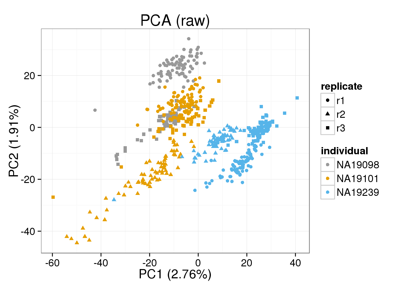

[[2]]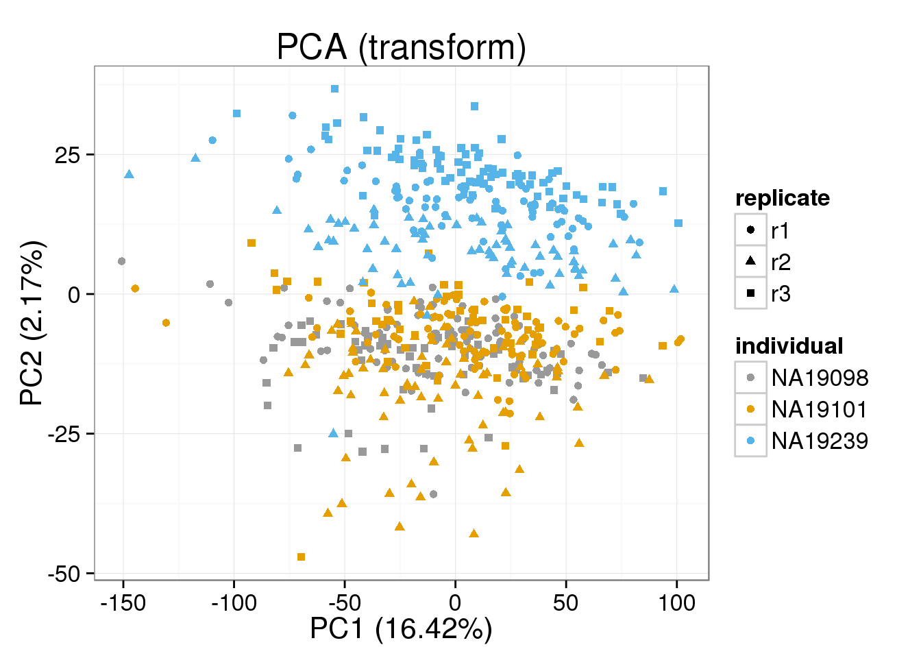

[[3]]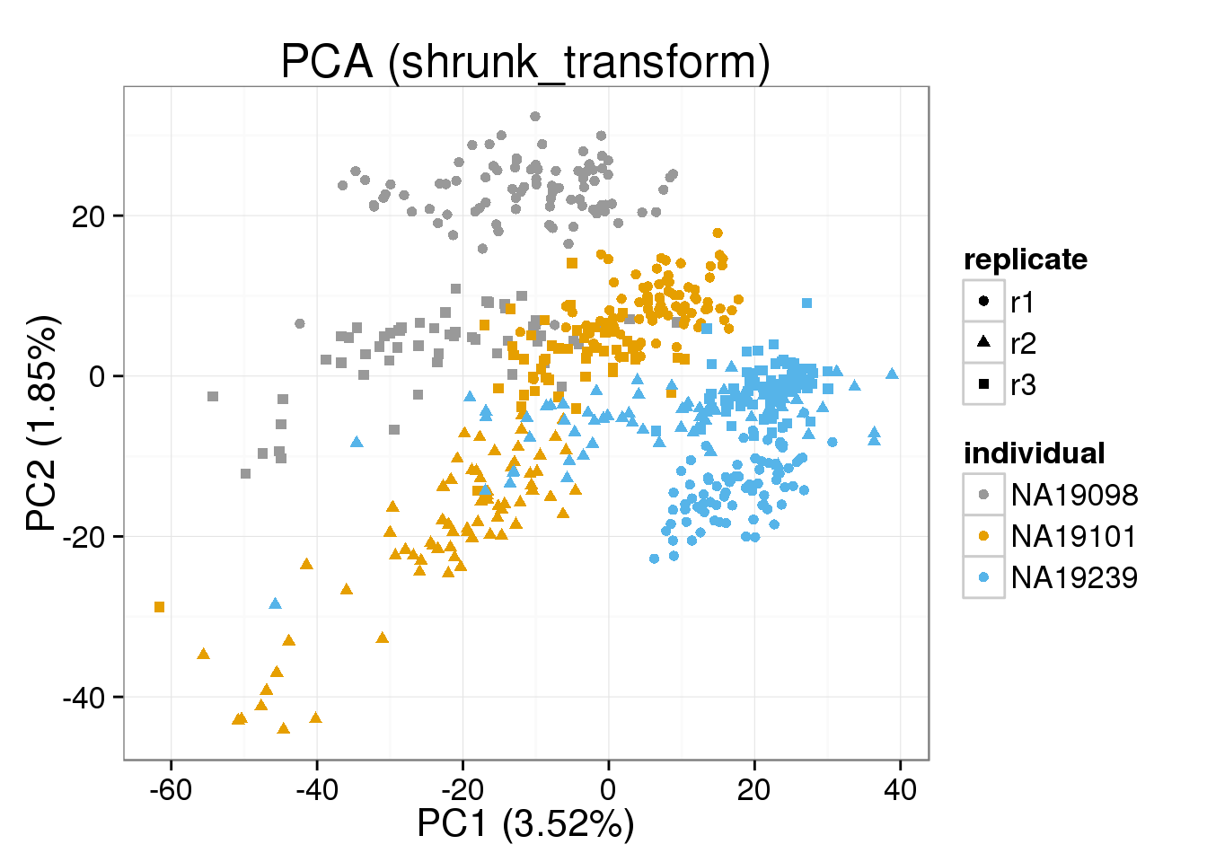

[[4]]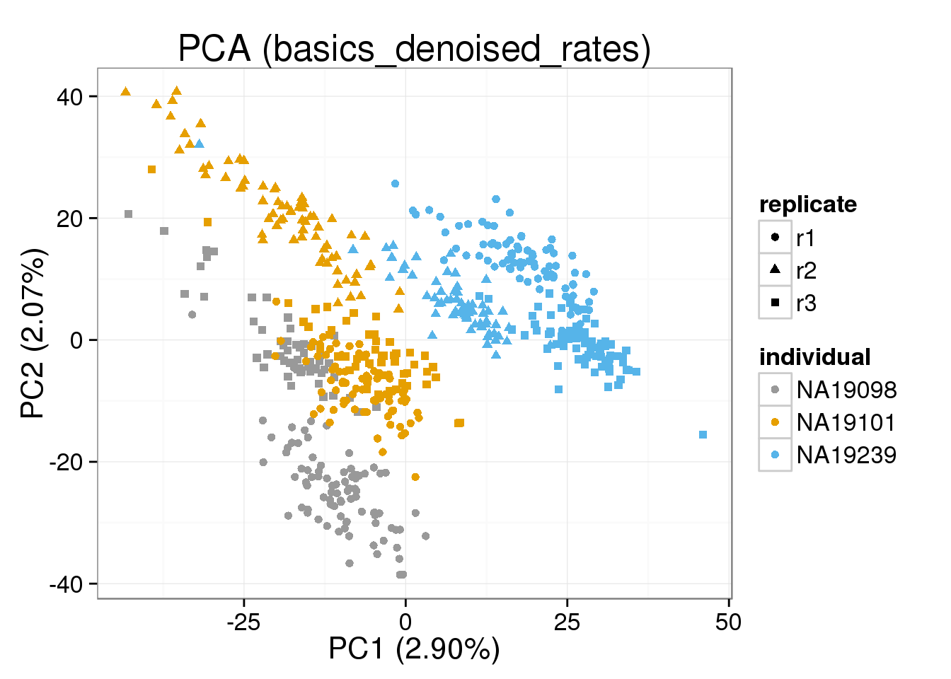

[[5]]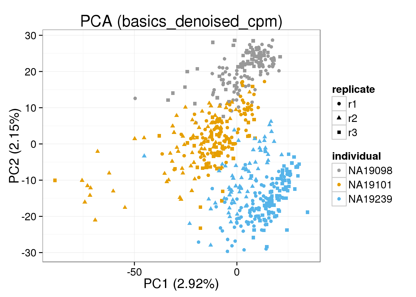

[[6]]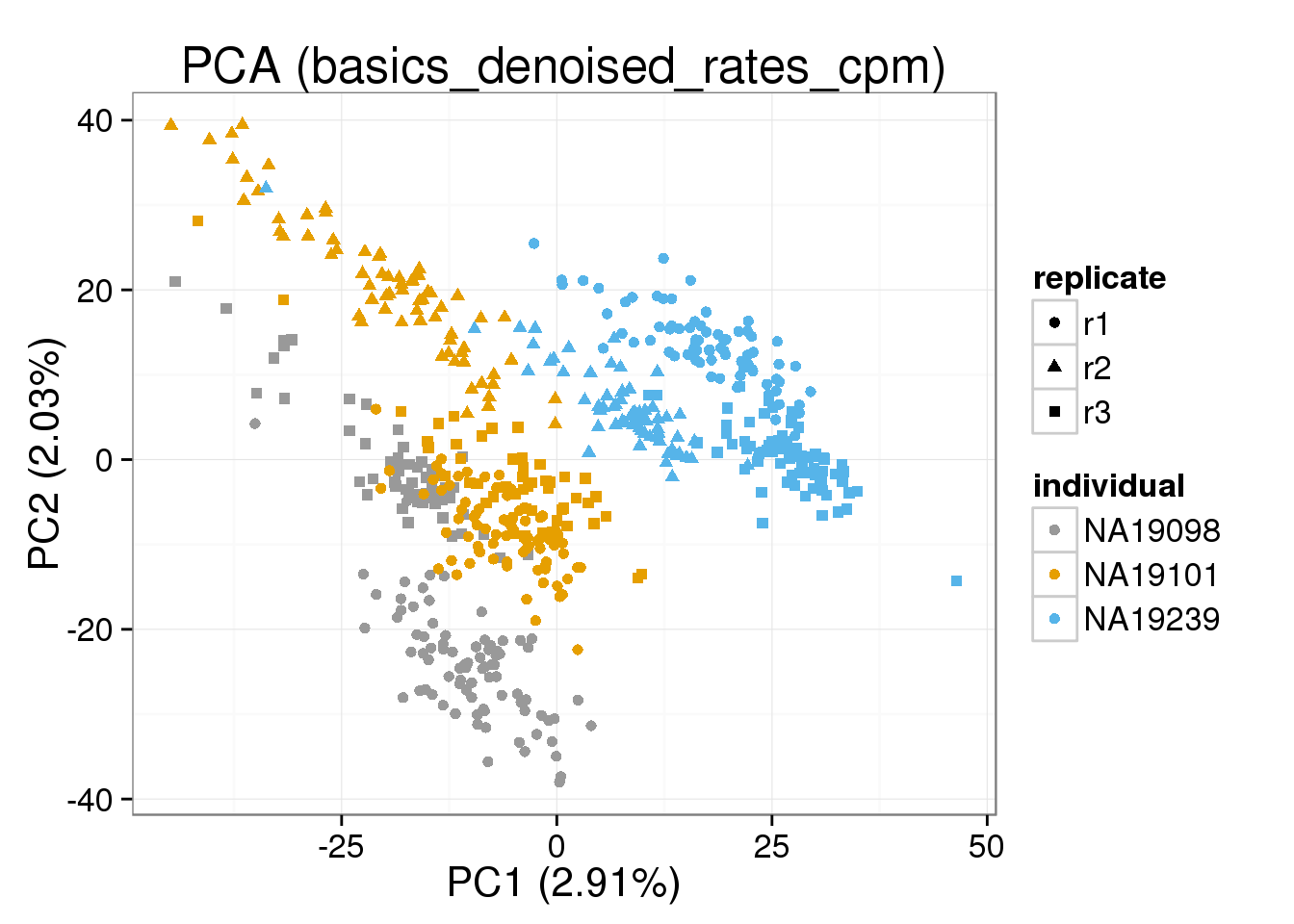

ANOVA

Next look at whether the batch and individual effects are more or less significant under the different normalization approaches using a per gene ANOVA.

anovas <- lapply(cpm_mats, function(x) {
  foreach(i=1:nrow(x)) %dopar% anova(lm(x[i,] ~ anno_filter$replicate + anno_filter$individual))
  })

variance_components <- lapply( as.list(names(anovas)), function(name) {
  ss=do.call(rbind,foreach(a=anovas[[name]]) %do% a[,"Sum Sq"] )
  colnames(ss)=c("batch","individual","residual")
  data.frame(sweep(ss,1,rowSums(ss),"/"), method=name)
} )
names(variance_components)=names(cpm_mats)

batch_over_explained <- lapply( as.list(names(anovas)), function(name) {
  ss=do.call(rbind,foreach(a=anovas[[name]]) %do% a[1:2,"Sum Sq"] )
  colnames(ss)=c("batch","individual")
  data.frame( prop_batch=ss[,"batch"] / rowSums(ss), method=name)
} )
names(batch_over_explained) = names(cpm_mats)

The histogram of the proportion explained by batch.

ggplot( do.call(rbind,batch_over_explained), aes(prop_batch,col=method)) + geom_density() + xlab("variance_batch / (variance_batch + variance_individual)")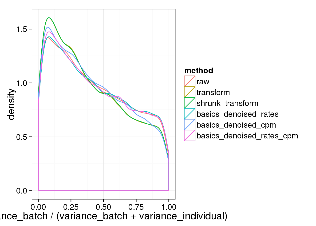

And the proportion of variance explained by either batch or individual.

ggplot( do.call(rbind,variance_components), aes(1-residual,col=method)) + geom_density() + xlab("proportion variance explained") + xlim(0,.5)+ scale_colour_manual(values=cbPalette)

Warning: Removed 25 rows containing non-finite values (stat_density).

Warning: Removed 15 rows containing non-finite values (stat_density).

Warning: Removed 25 rows containing non-finite values (stat_density).

Warning: Removed 29 rows containing non-finite values (stat_density).

Warning: Removed 26 rows containing non-finite values (stat_density).

Warning: Removed 28 rows containing non-finite values (stat_density).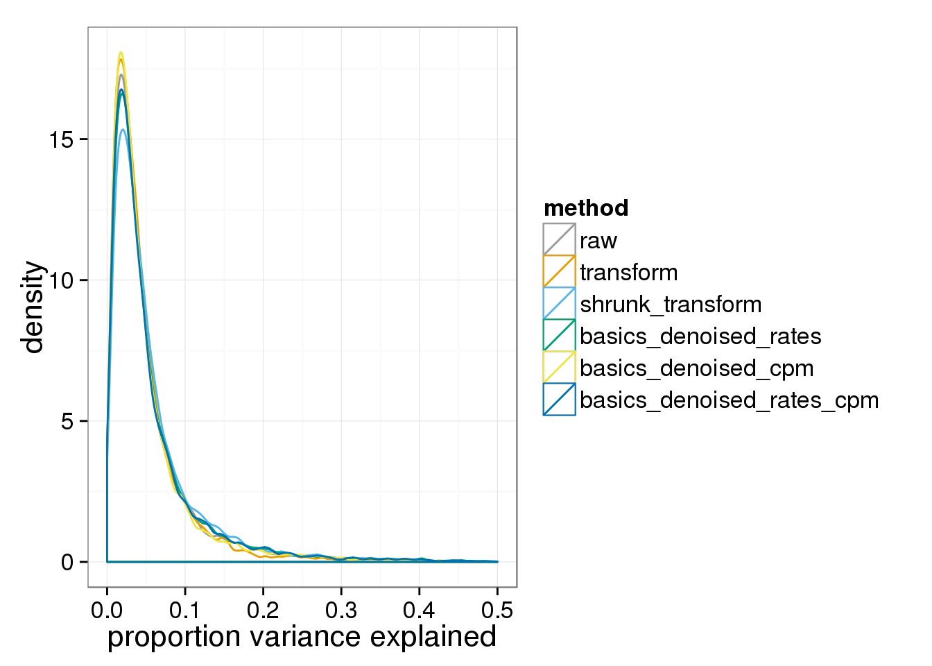

Any version of the BASICS normalized data behaves basically (sic) like the raw data.