Compare read and molecule counts per batch

Input
Filter
Transformation
Differences in conversion of reads to molecules
Comparing loess curves
Session information

Last updated: 2015-09-08

Code version: 7ac0a8c74137d15731f4b4c1ab6acd4f21d2f8bd

Comparing the conversion of reads to molecules for each of the 9 batches. Used three different metrics:

Raw counts
Log2 counts (pseudocount of 1)
Log2 TMM-normalized counts per million (pseudocount of 0.25)

Input

library("dplyr")
library("ggplot2")
theme_set(theme_bw(base_size = 16))
library("edgeR")
source("functions.R")
library("tidyr")

Input annotation.

anno <- read.table("../data/annotation.txt", header = TRUE,
                   stringsAsFactors = FALSE)
head(anno)

  individual batch well     sample_id
1      19098     1  A01 NA19098.1.A01
2      19098     1  A02 NA19098.1.A02
3      19098     1  A03 NA19098.1.A03
4      19098     1  A04 NA19098.1.A04
5      19098     1  A05 NA19098.1.A05
6      19098     1  A06 NA19098.1.A06

Input read counts.

reads <- read.table("../data/reads.txt", header = TRUE,
                    stringsAsFactors = FALSE)

Input molecule counts.

molecules <- read.table("../data/molecules.txt", header = TRUE,
                    stringsAsFactors = FALSE)

Input list of quality single cells.

quality_single_cells <- scan("../data/quality-single-cells.txt",
                             what = "character")

Filter

Keep only the single cells that passed the QC filters.

reads <- reads[, colnames(reads) %in% quality_single_cells]
molecules <- molecules[, colnames(molecules) %in% quality_single_cells]
anno <- anno[anno$sample_id %in% quality_single_cells, ]
stopifnot(dim(reads) == dim(molecules),
          nrow(anno) == ncol(reads))

Only keep the following genes:

ERCC genes with at least one molecule observed in at least one single cell

ercc_keep <- rownames(molecules)[grepl("ERCC", rownames(molecules)) &
                                 rowSums(molecules) > 1]

The top expressed endogenous genes in terms of mean molecule counts per million

num_genes <- 12000
mean_cpm <- molecules %>%
  filter(!grepl("ERCC", rownames(molecules))) %>%
  cpm %>%
  rowMeans
gene_keep <- rownames(molecules)[!grepl("ERCC", rownames(molecules))][order(mean_cpm, decreasing = TRUE)][1:num_genes]

Filter the genes:

reads <- reads[rownames(reads) %in% c(gene_keep, ercc_keep), ]
molecules <- molecules[rownames(molecules) %in% c(gene_keep, ercc_keep), ]

Transformation

In addition to comparing the raw counts of reads and molecules, we compare the log2 counts and the log counts per million.

For the log counts, I add a pseudocount of 1.

reads_log <- log2(reads + 1)
molecules_log <- log2(molecules + 1)

Calculate cpm for the reads data using TMM-normalization.

norm_factors_reads <- calcNormFactors(reads, method = "TMM")
reads_cpm <- cpm(reads, lib.size = colSums(reads) * norm_factors_reads,
                 log = TRUE)

And for the molecules.

norm_factors_mol <- calcNormFactors(molecules, method = "TMM")
molecules_cpm <- cpm(molecules, lib.size = colSums(molecules) * norm_factors_mol,
                     log = TRUE)

Differences in conversion of reads to molecules

As seen above with the total counts, the conversion of reads to molecules varies between each of the 9 batches. Below I fit a loess transformation to each individually. It would be ideal if we could somehow we could correct for these differences and have them all follow a similar transformation from reads to molecules.

convert_to_long <- function(r, m) {
  # Combines reads and molecules into long format for comparison of conversion
  #
  # r - reads in wide format
  # m - molecules in wide format
  r <- data.frame(gene = rownames(r), r)
  m <- data.frame(gene = rownames(m), m)
  r_long <- gather_(r, key = "id", value = "reads",
                    grep("NA", colnames(r), value = TRUE))
  m_long <- gather_(m, key = "id", value = "molecules",
                    grep("NA", colnames(m), value = TRUE))
  r_long <- separate_(r_long, col = "id",  sep = "\\.", remove = FALSE,
                     into = c("individual", "batch", "well"))
  stopifnot(r_long$id == m_long$id,
            r_long$gene == m_long$gene)
  conversion <- cbind(r_long, m_long$molecules)
  colnames(conversion)[ncol(conversion)] <- "molecules"
  stopifnot(nrow(conversion) == nrow(m_long))
  return(conversion)
}

In order to be able to make this plot, I have to subsample to fewer genes. Otherwise it runs out of memory.

set.seed(12345)
num_subsampled <- 5000
sub_indices <- sample(1:nrow(reads), num_subsampled)
# counts
reads_sub <- reads[sub_indices, ]
molecules_sub <- molecules[sub_indices, ]
# log counts
reads_log_sub <- reads_log[sub_indices, ]
molecules_log_sub <- molecules_log[sub_indices, ]
# log counts per million
reads_cpm_sub <- reads_cpm[sub_indices, ]
molecules_cpm_sub <- molecules_cpm[sub_indices, ]
# Convert to long format
conversion <- convert_to_long(reads_sub, molecules_sub)
conversion_log <- convert_to_long(reads_log_sub, molecules_log_sub)
conversion_cpm <- convert_to_long(reads_cpm_sub, molecules_cpm_sub)
head(conversion)

             gene            id individual batch well reads molecules
1 ENSG00000118777 NA19098.1.A01    NA19098     1  A01     0         0
2 ENSG00000157800 NA19098.1.A01    NA19098     1  A01     2         2
3 ENSG00000168944 NA19098.1.A01    NA19098     1  A01     0         0
4 ENSG00000158941 NA19098.1.A01    NA19098     1  A01   198         4
5 ENSG00000167671 NA19098.1.A01    NA19098     1  A01     0         0
6 ENSG00000171219 NA19098.1.A01    NA19098     1  A01     0         0

Summarize across the single cells for each of the 9 batches.

# counts
conversion_mean <- conversion %>%
  filter(well != "bulk") %>%
  group_by(individual, batch, gene) %>%
  summarize(reads_mean = mean(reads),
            reads_sem = sd(reads) / sqrt(length(reads)),
            molecules_mean = mean(molecules),
            molecules_sem = sd(molecules) / sqrt(length(molecules)))
# log counts
conversion_log_mean <- conversion_log %>%
  filter(well != "bulk") %>%
  group_by(individual, batch, gene) %>%
  summarize(reads_mean = mean(reads),
            reads_sem = sd(reads) / sqrt(length(reads)),
            molecules_mean = mean(molecules),
            molecules_sem = sd(molecules) / sqrt(length(molecules)))

# counts per million
conversion_cpm_mean <- conversion_cpm %>%
  filter(well != "bulk") %>%
  group_by(individual, batch, gene) %>%
  summarize(reads_mean = mean(reads),
            reads_sem = sd(reads) / sqrt(length(reads)),
            molecules_mean = mean(molecules),
            molecules_sem = sd(molecules) / sqrt(length(molecules)))
head(conversion_cpm_mean)

Source: local data frame [6 x 7]
Groups: individual, batch

  individual batch            gene reads_mean reads_sem molecules_mean
1    NA19098     1 ENSG00000000457 -0.8607341 0.3575195       2.574378
2    NA19098     1 ENSG00000000460  2.7123079 0.3738981       4.629304
3    NA19098     1 ENSG00000001460  0.4673185 0.3861463       3.414075
4    NA19098     1 ENSG00000001617 -1.7289385 0.2945758       2.027832
5    NA19098     1 ENSG00000002016 -2.0541566 0.2846078       1.898482
6    NA19098     1 ENSG00000002549  3.9782091 0.3088070       5.525236
Variables not shown: molecules_sem (dbl)

Counts

Compare the counts.

conver_plot_counts <- ggplot(conversion_mean,
                             aes(x = reads_mean, y = molecules_mean, col = individual,
                                 shape = as.factor(batch))) +
  geom_point() +
  geom_errorbar(aes(ymin = molecules_mean - molecules_sem,
                    ymax = molecules_mean + molecules_sem)) +
  geom_errorbarh(aes(xmin = reads_mean - reads_sem,
                     xmax = reads_mean + reads_sem)) +
  geom_smooth(method = "loess", color = "black") +
  facet_grid(batch ~ individual) +
  theme(legend.position = "none") +
  labs(x = "Reads per gene",
       y = "Molecules per gene",
       title = sprintf("Conversion per batch (subsample of %d genes)", num_subsampled))
conver_plot_counts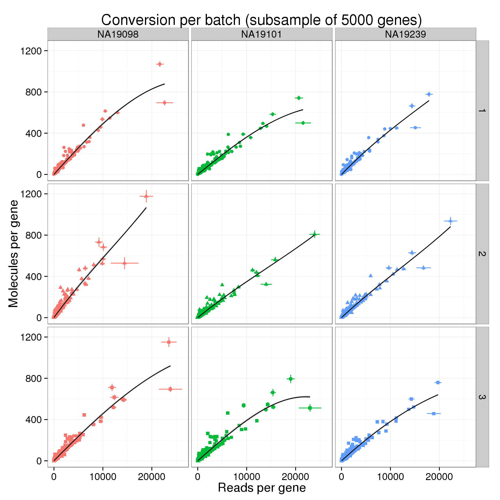

Log2 counts

Compare the log counts.

conver_plot_log <- conver_plot_counts %+%
  conversion_log_mean +
  geom_line(aes(x = reads_mean, y = reads_mean)) +
  labs(x = "Reads per gene (log2)",
       y = "Molecules per gene (log2)",
       title = sprintf("Conversion per batch (subsample of %d genes) - log", num_subsampled))
conver_plot_log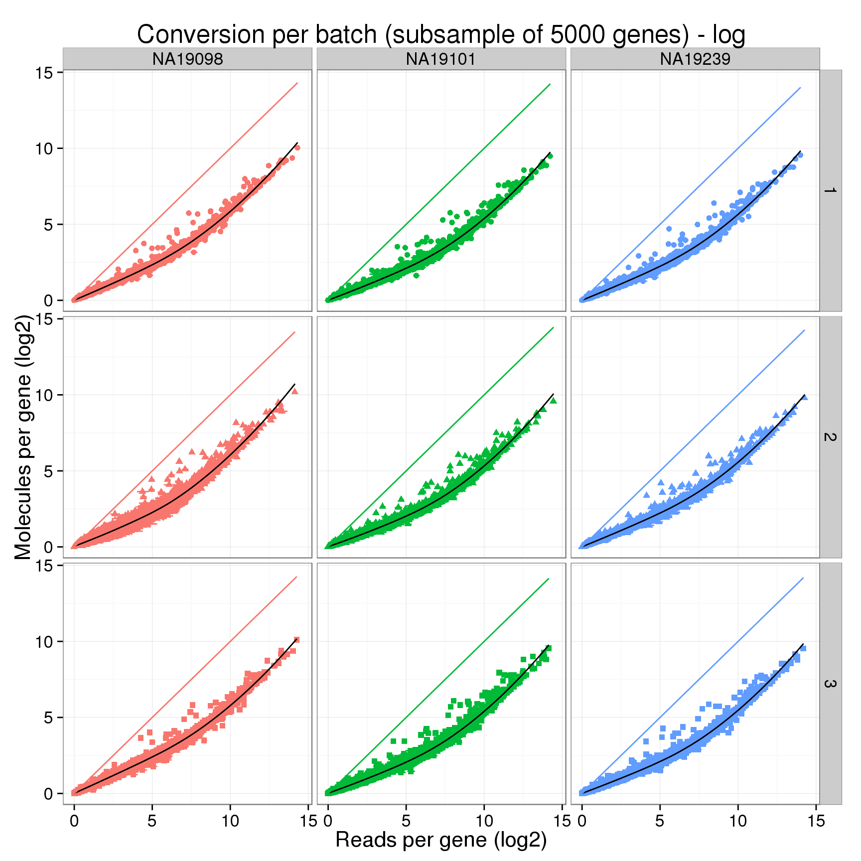

Log2 counts per million

Compare the counts per million.

conver_plot_cpm <- conver_plot_log %+%
  conversion_cpm_mean +
  labs(x = "Reads per million per gene (log2)",
       y = "Molecules per million per gene (log2)",
       title = sprintf("Conversion per batch (subsample of %d genes) - cpm", num_subsampled))
conver_plot_cpm + geom_line(aes(x = reads_mean, y = reads_mean))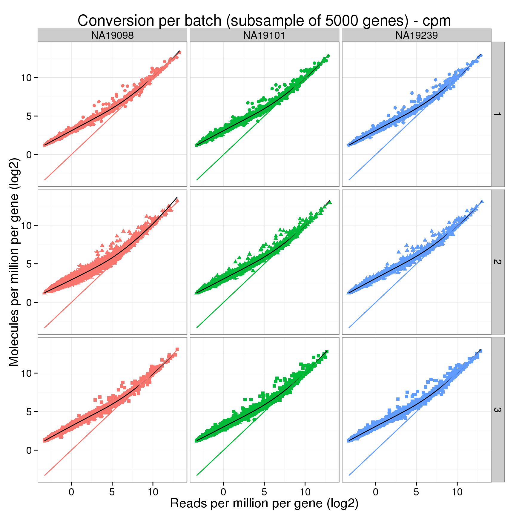

Now visualizing only the ERCC.

conversion_ercc <- convert_to_long(reads[grep("ERCC", rownames(reads)), ],
                                   molecules[grep("ERCC", rownames(molecules)), ])
conversion_ercc_log <- convert_to_long(reads_log[grep("ERCC", rownames(reads_log)), ],
                                       molecules_log[grep("ERCC", rownames(molecules_log)), ])
conversion_ercc_cpm <- convert_to_long(reads_cpm[grep("ERCC", rownames(reads_cpm)), ],
                                       molecules_cpm[grep("ERCC", rownames(molecules_cpm)), ])
# Remove 19098 batch 2 because the outlier throws off the axes
conversion_ercc <- conversion_ercc[!(conversion_ercc$individual == "NA19098" &
                                     conversion_ercc$batch == 2), ]
conversion_ercc_log <- conversion_ercc_log[!(conversion_ercc_log$individual == "NA19098" &
                                             conversion_ercc_log$batch == 2), ]
conversion_ercc_cpm <- conversion_ercc_cpm[!(conversion_ercc_cpm$individual == "NA19098" &
                                             conversion_ercc_cpm$batch == 2), ]

# counts
conversion_ercc_mean <- conversion_ercc %>%
  filter(well != "bulk") %>%
  group_by(individual, batch, gene) %>%
  summarize(reads_mean = mean(reads),
         reads_sem = sd(reads) / sqrt(length(reads)),
         molecules_mean = mean(molecules),
         molecules_sem = sd(molecules) / sqrt(length(molecules)))
# log counts
conversion_ercc_log_mean <- conversion_ercc_log %>%
  filter(well != "bulk") %>%
  group_by(individual, batch, gene) %>%
  summarize(reads_mean = mean(reads),
         reads_sem = sd(reads) / sqrt(length(reads)),
         molecules_mean = mean(molecules),
         molecules_sem = sd(molecules) / sqrt(length(molecules)))
# counts per million
conversion_ercc_cpm_mean <- conversion_ercc_cpm %>%
  filter(well != "bulk") %>%
  group_by(individual, batch, gene) %>%
  summarize(reads_mean = mean(reads),
         reads_sem = sd(reads) / sqrt(length(reads)),
         molecules_mean = mean(molecules),
         molecules_sem = sd(molecules) / sqrt(length(molecules)))
head(conversion_ercc_cpm_mean)

Source: local data frame [6 x 7]
Groups: individual, batch

  individual batch       gene reads_mean    reads_sem molecules_mean
1    NA19098     1 ERCC-00002  11.443245 7.161031e-02      11.357225
2    NA19098     1 ERCC-00003   7.789998 1.437894e-01       7.802351
3    NA19098     1 ERCC-00004   9.740596 8.954873e-02       9.725388
4    NA19098     1 ERCC-00009   6.684334 1.715310e-01       6.895313
5    NA19098     1 ERCC-00012  -3.253281 3.527606e-02       1.267489
6    NA19098     1 ERCC-00013  -3.303453 2.878603e-17       1.218331
Variables not shown: molecules_sem (dbl)

ERCC counts

conver_plot_ercc <- conver_plot_counts %+%
  conversion_ercc_mean +
  labs(title = "Conversion per batch (ERCC genes)")
conver_plot_ercc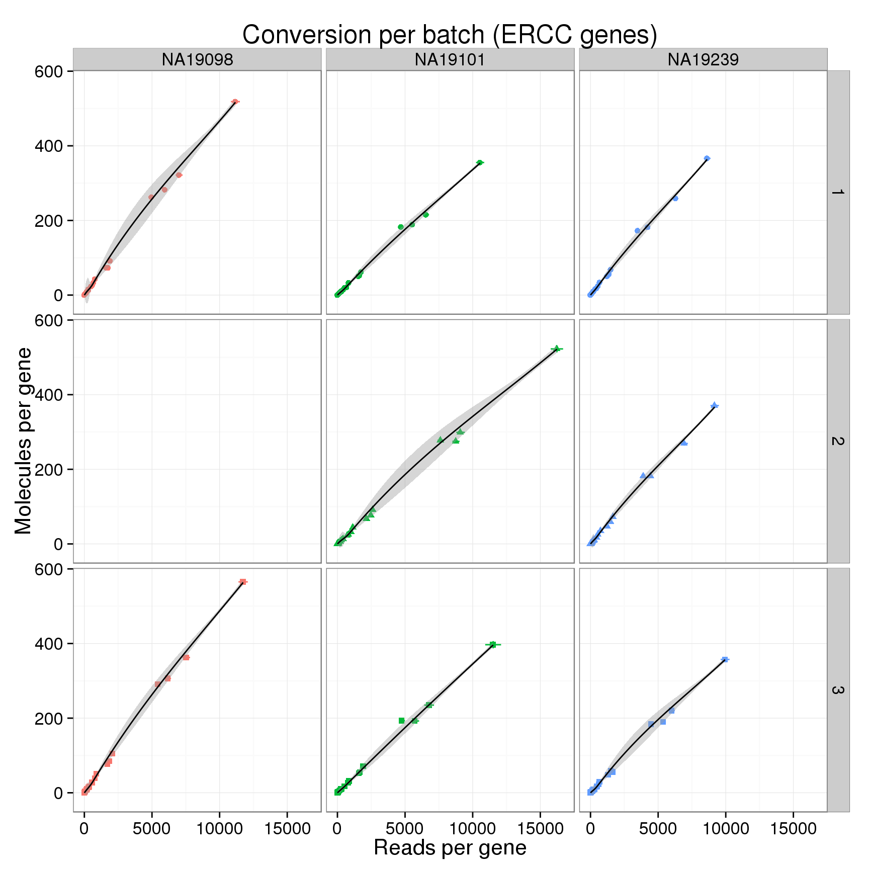

ERCC log2 counts

conver_plot_ercc_log <- conver_plot_log %+%
  conversion_ercc_log_mean +
  labs(x = "Reads per million per gene (log2)",
       y = "Molecules per million per gene (log2)",
       title = "Conversion per batch (ERCC genes) - log")
conver_plot_ercc_log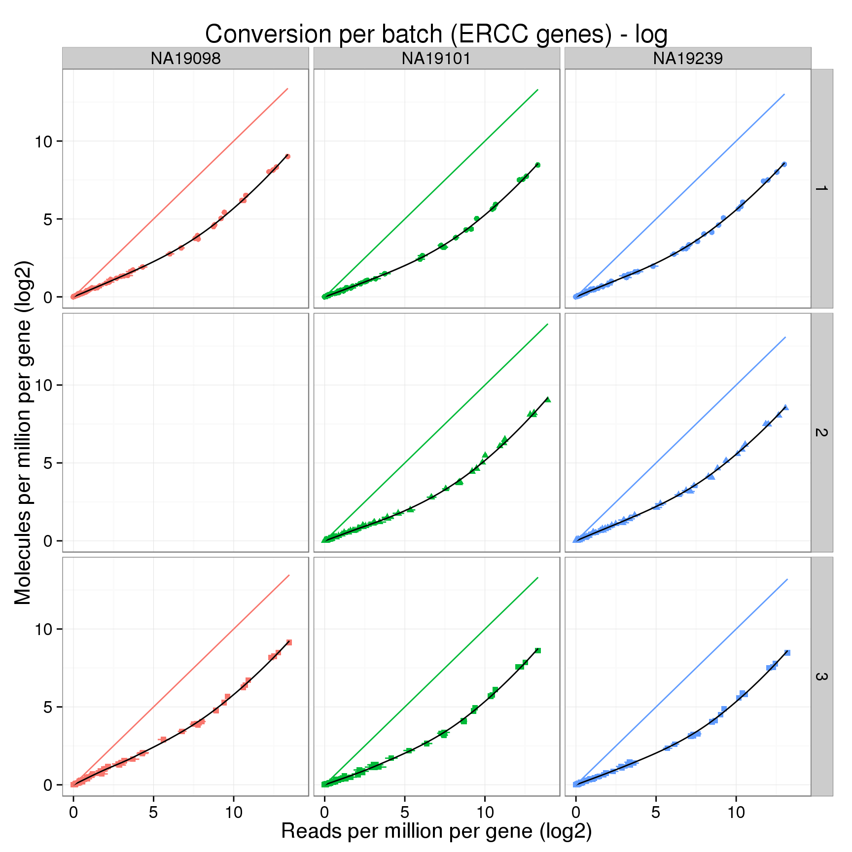

ERCC log2 counts per million

conver_plot_ercc_cpm <- conver_plot_log %+%
  conversion_ercc_cpm_mean +
  labs(x = "Reads per million per gene",
       y = "Molecules per million per gene",
       title = "Conversion per batch (ERCC genes) - cpm")
conver_plot_ercc_cpm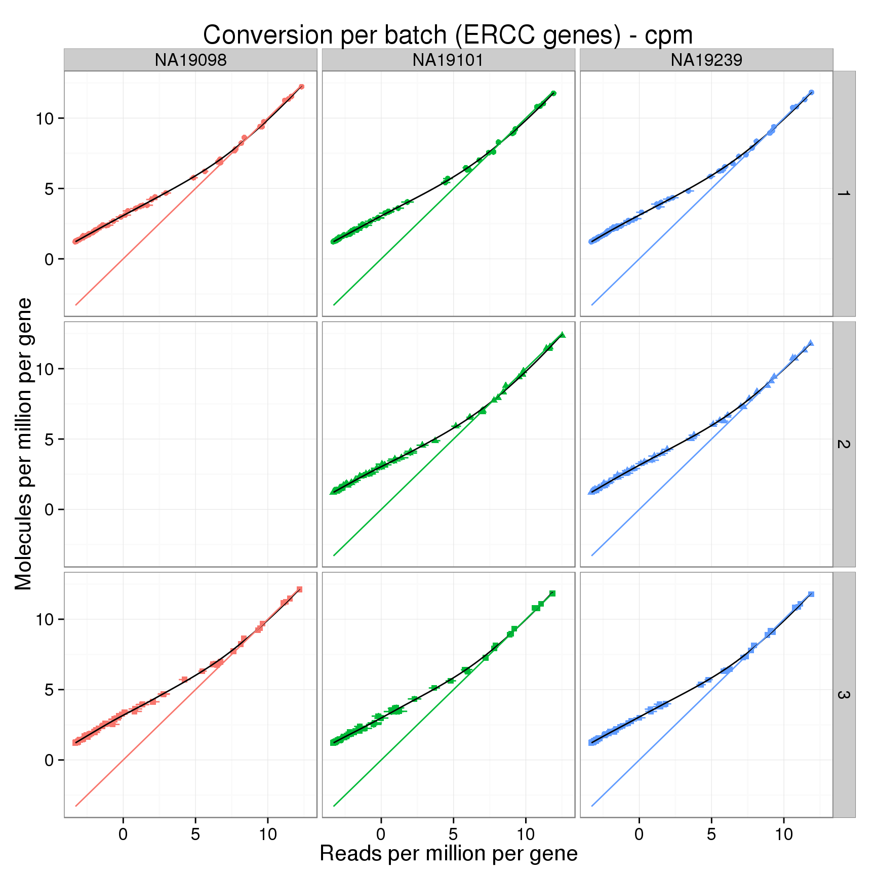

Comparing loess curves

Can we identify batch effects in the conversion of reads to molecules by closely comparing the loess fits? Below I calculate two statistics for the log2 cpm data. The first is the maximum absolute difference between the loess curve and the line y=x. The largest differences are observed for the lowly expressed genes. The second is the x-coordinate (the mean number of log2 reads per million per gene) where the loess curve and the line y=x intersect.

The first section below is simply the code I used to explore one batch.

conversion_chunk <- filter(conversion_cpm_mean, individual == "NA19101", batch == 1)
dim(conversion_chunk)

[1] 5000    7

head(conversion_chunk)

Source: local data frame [6 x 7]
Groups: individual, batch

  individual batch            gene reads_mean reads_sem molecules_mean
1    NA19101     1 ENSG00000000457 -2.2707890 0.2789448       1.834098
2    NA19101     1 ENSG00000000460  1.9943078 0.4270220       4.262028
3    NA19101     1 ENSG00000001460  0.2033697 0.4061393       3.319563
4    NA19101     1 ENSG00000001617 -1.6354899 0.3198890       2.124191
5    NA19101     1 ENSG00000002016 -0.4858941 0.4056412       2.869652
6    NA19101     1 ENSG00000002549  5.0039819 0.2831578       5.990995
Variables not shown: molecules_sem (dbl)

loess_model <- loess(molecules_mean ~ reads_mean, data = conversion_chunk)
loess_predict <- predict(loess_model)
str(loess_predict)

 num [1:5000] 1.82 4.22 3.22 2.18 2.83 ...

plot(conversion_chunk$reads_mean, loess_predict)
abline(a = 0, b = 1, col = "red")

plot(conversion_chunk$molecules_mean, loess_predict)

plot(conversion_chunk$reads_mean, conversion_chunk$reads_mean - loess_predict)
abline(h = 0, col = "red")

max(abs(conversion_chunk$reads_mean - loess_predict))

[1] 4.528132

Here are the functions I used.

predict_loess <- function(x, y) {
  # Perform loess regression and return the predicted y-values.
  model <- loess(y ~ x)
  prediction <- predict(model)
  return(prediction)
}
find_max_loess_diff <- function(x, y) {
  # Find the maximum absolute difference between the loess curve and the line
  # y=x.
  y_predict <- predict_loess(x, y)
  max_loess_diff <- max(abs(x - y_predict))
  return(max_loess_diff)
}
find_loess_intersect <- function(x, y) {
  # Find the x-coordinate where the loess curve and the line y=x intersect.
  y_predict <- predict_loess(x, y)
  x_order <- order(x)
  x <- x[x_order]
  y_predict <- y_predict[x_order]
  loess_diffs <- y_predict - x
  intersection <- x[loess_diffs <= 0][1]
  return(intersection)
}
find_max_loess_diff(conversion_chunk$reads_mean, conversion_chunk$molecules_mean)

[1] 4.528132

find_loess_intersect(conversion_chunk$reads_mean, conversion_chunk$molecules_mean)

[1] 9.093351

These are the results for 5000 randomly subsampled genes (include endegenous genes and some ERCC).

batch_loess <- conversion_cpm_mean %>%
  group_by(individual, batch) %>%
  summarize(max_loess_diff = find_max_loess_diff(reads_mean, molecules_mean),
            loess_intersect = find_loess_intersect(reads_mean, molecules_mean))
batch_loess

Source: local data frame [9 x 4]
Groups: individual

  individual batch max_loess_diff loess_intersect
1    NA19098     1       4.526934              NA
2    NA19098     2       4.557171              NA
3    NA19098     3       4.524544        8.909048
4    NA19101     1       4.528132        9.093351
5    NA19101     2       4.535132        9.102370
6    NA19101     3       4.533278        9.750998
7    NA19239     1       4.524167        9.519240
8    NA19239     2       4.526112        9.202881
9    NA19239     3       4.524408        9.695773

These are the results for the ERCC alone.

batch_loess_ercc <- conversion_ercc_cpm_mean %>%
  group_by(individual, batch) %>%
  summarize(max_loess_diff = find_max_loess_diff(reads_mean, molecules_mean),
            loess_intersect = find_loess_intersect(reads_mean, molecules_mean))
batch_loess_ercc

Source: local data frame [8 x 4]
Groups: individual

  individual batch max_loess_diff loess_intersect
1    NA19098     1       4.523076        9.489872
2    NA19098     3       4.519575        9.341845
3    NA19101     1       4.522796        9.097392
4    NA19101     2       4.517937        7.811393
5    NA19101     3       4.520843        9.204111
6    NA19239     1       4.515316        9.051180
7    NA19239     2       4.522820        9.343531
8    NA19239     3       4.521505        8.883230

Session information

sessionInfo()

R version 3.2.0 (2015-04-16)
Platform: x86_64-unknown-linux-gnu (64-bit)

locale:
 [1] LC_CTYPE=en_US.UTF-8       LC_NUMERIC=C              
 [3] LC_TIME=en_US.UTF-8        LC_COLLATE=en_US.UTF-8    
 [5] LC_MONETARY=en_US.UTF-8    LC_MESSAGES=en_US.UTF-8   
 [7] LC_PAPER=en_US.UTF-8       LC_NAME=C                 
 [9] LC_ADDRESS=C               LC_TELEPHONE=C            
[11] LC_MEASUREMENT=en_US.UTF-8 LC_IDENTIFICATION=C       

attached base packages:
[1] stats     graphics  grDevices utils     datasets  methods   base     

other attached packages:
[1] tidyr_0.2.0   edgeR_3.10.2  limma_3.24.9  ggplot2_1.0.1 dplyr_0.4.2  
[6] knitr_1.10.5 

loaded via a namespace (and not attached):
 [1] Rcpp_0.12.0      magrittr_1.5     MASS_7.3-40      munsell_0.4.2   
 [5] colorspace_1.2-6 R6_2.1.1         stringr_1.0.0    plyr_1.8.3      
 [9] tools_3.2.0      parallel_3.2.0   grid_3.2.0       gtable_0.1.2    
[13] DBI_0.3.1        htmltools_0.2.6  lazyeval_0.1.10  yaml_2.1.13     
[17] assertthat_0.1   digest_0.6.8     reshape2_1.4.1   formatR_1.2     
[21] codetools_0.2-11 evaluate_0.7     rmarkdown_0.6.1  labeling_0.3    
[25] stringi_0.4-1    scales_0.2.4     proto_0.3-10