Coverage of ERCC spike-ins

Input
Prepare data
Calculate coverage
Summarize coverage
Metagene plot
Interpretation
Session information

Last updated: 2016-02-22

Code version: c583b1dbf009e01374eca3103be81ca554fd7fb1

This is a companion to the analysis of the coverage of endogenous genes. It must be run first to prepare the bam files. We do not observe the expected 5’ bias of the UMI protocol for the ERCC spike-ins.

library("genomation")
library("plyr")
library("tidyr")
library("ggplot2")
theme_set(theme_bw(base_size = 14))
theme_update(panel.grid.minor.x = element_blank(),
             panel.grid.minor.y = element_blank(),
             panel.grid.major.x = element_blank(),
             panel.grid.major.y = element_blank())

Input

Input filtered molecule counts.

molecules_filter <- read.table("../data/molecules-filter.txt", header = TRUE,
                               stringsAsFactors = FALSE)
molecules_ercc <- molecules_filter[grep("ERCC", rownames(molecules_filter)), ]

Input ERCC data from Invitrogen.

ercc_all <- gffToGRanges("../data/ERCC92.gtf", split.group = TRUE)

splitting the group.column...

Prepare data

Filter the ERCC spike-ins to only include those that pass the filter.

ercc_filter <- ercc_all[ercc_all$gene_id %in% rownames(molecules_ercc)]

Create subset that only include 5 most highly expressed ERCC spike-ins.

# Order by mean expression - from highest to lowest
mean_expr_ercc <- rowMeans(molecules_ercc)
molecules_ercc <- molecules_ercc[order(mean_expr_ercc, decreasing = TRUE), ]
ercc_max <- ercc_filter[ercc_filter$gene_id %in% rownames(molecules_ercc)[1:5]]

Using the same quality single cell samples from the analysis of the coverage of endogenous genes.

quality_cells <- c("19098.1.A01", "19101.1.A02", "19239.1.A01")
names(quality_cells) <- c("NA19098.r1.A01", "NA19101.r1.A02", "NA19239.r1.A01")
stopifnot(names(quality_cells) %in% colnames(molecules_filter))
bam <- paste0("../data/", quality_cells, ".trim.sickle.sorted.combined.rmdup.sorted.bam")
stopifnot(file.exists(bam), file.exists(paste0(bam, ".bai")))

Calculate coverage

Because the ERCC have different lengths, we have to bin them. ScoreMatrix and ScoreMatrixList handle one or multiple files, respectively, and calculate the coverage over windows of equal size. ScoreMatrixBin computes the coverage of one file over windows of unequal size. For some reason, ScoreMatrixBinList does not exist (here is an old issue from 2013 that discusses adding the feature for ScoreMatrix only). Thus we loop over the files manually.

filter_sm <- list()
for (b in bam) {
  filter_sm[[b]] <- ScoreMatrixBin(target = b, windows = ercc_filter, type = "bam",
                                   rpm = TRUE, strand.aware = TRUE, bin.num = 50)
}

Normalizing to rpm ...
Normalizing to rpm ...
Normalizing to rpm ...

filter_sm <- new("ScoreMatrixList", .Data = filter_sm)

Calculate coverage for only the 5 most highly expressed ERCC.

max_sm <- list()
for (b in bam) {
  max_sm[[b]] <- ScoreMatrixBin(target = b, windows = ercc_max, type = "bam",
                                   rpm = TRUE, strand.aware = TRUE, bin.num = 50)
}

Normalizing to rpm ...
Normalizing to rpm ...
Normalizing to rpm ...

max_sm <- new("ScoreMatrixList", .Data = max_sm)

Summarize coverage

names(filter_sm) <- names(quality_cells)
filter_sm_df <- ldply(filter_sm, colMeans, .id = "sample_id")
colnames(filter_sm_df)[-1] <- paste0("p", 1:(ncol(filter_sm_df) - 1))
filter_sm_df$subset = "filter"
filter_sm_df_long <- gather(filter_sm_df, key = "pos", value = "rpm", p1:p50)

names(max_sm) <- names(quality_cells)
max_sm_df <- ldply(max_sm, colMeans, .id = "sample_id")
colnames(max_sm_df)[-1] <- paste0("p", 1:(ncol(max_sm_df) - 1))
max_sm_df$subset = "max"
max_sm_df_long <- gather(max_sm_df, key = "pos", value = "rpm", p1:p50)

Combine the two features.

features <- rbind(filter_sm_df_long, max_sm_df_long)
# Convert base position back to integer value
features$pos <- sub("p", "", features$pos)
features$pos <- as.numeric(features$pos)
# Make subset factor more descriptive
features$subset <- factor(features$subset, levels = c("filter", "max"),
                          labels = c(paste(length(ercc_filter), "ERCC that pass expression filter"),
                                     "5 most abundant ERCC"))

Metagene plot

ggplot(features, aes(x = pos, y = rpm, color = sample_id)) +
  geom_line() +
  facet_wrap(~subset) + 
  scale_color_discrete(name = "Sample") +
  labs(x = "Bins (50) 5' -> 3'",
       y = "Counts per million (mean)",
       title = "5' bias of UMI protocol????") +
  theme(legend.position = "bottom")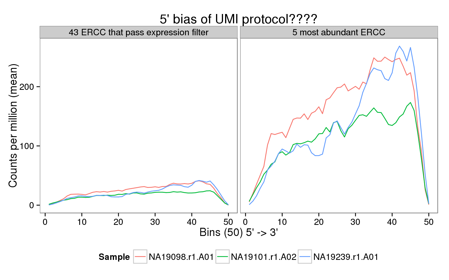

Interpretation

This was an unexpected result. There appears to be more coverage on the 3’ end of the ERCC spike-ins. Some potential explanations:

The GTF file lists the ERCC as on the positive strand. Maybe this needs to be switched (genomation does not filter reads based on strand). However, I checked (example code below) and this is not the case. The reads are mapped to the positive strand.

samtools view ../data/19098.1.A01.trim.sickle.sorted.combined.rmdup.sorted.bam -c -F 1x10 ERCC-00002

We saw in the coverage of the endogenous genes that many molecules mapped just upstream of the TSS. Maybe there is some issue with the template switching, so that many reads do not get mapped to the 5’ of the ERCC?
Maybe it could be a length issue? If a the transcript length is short, then the cumulative coverage at the 3’ end could be higher than it should. However, running it with only the 19 ERCC that pass the filter and are longer than 1 kb (ercc_filter@ranges@width > 1000) did not change the overall pattern. The only difference was that NA19098 had a more noticeable peak at the 5’ end, but it was still less than the 3’ end.

Session information

sessionInfo()

R version 3.2.0 (2015-04-16)
Platform: x86_64-unknown-linux-gnu (64-bit)

locale:
 [1] LC_CTYPE=en_US.UTF-8       LC_NUMERIC=C              
 [3] LC_TIME=en_US.UTF-8        LC_COLLATE=en_US.UTF-8    
 [5] LC_MONETARY=en_US.UTF-8    LC_MESSAGES=en_US.UTF-8   
 [7] LC_PAPER=en_US.UTF-8       LC_NAME=C                 
 [9] LC_ADDRESS=C               LC_TELEPHONE=C            
[11] LC_MEASUREMENT=en_US.UTF-8 LC_IDENTIFICATION=C       

attached base packages:
[1] grid      stats     graphics  grDevices utils     datasets  methods  
[8] base     

other attached packages:
[1] ggplot2_1.0.1    tidyr_0.2.0      plyr_1.8.3       genomation_1.0.0
[5] knitr_1.10.5    

loaded via a namespace (and not attached):
 [1] Rcpp_0.12.0             formatR_1.2            
 [3] futile.logger_1.4.1     GenomeInfoDb_1.4.0     
 [5] XVector_0.8.0           bitops_1.0-6           
 [7] futile.options_1.0.0    tools_3.2.0            
 [9] zlibbioc_1.14.0         digest_0.6.8           
[11] evaluate_0.7            gtable_0.1.2           
[13] gridBase_0.4-7          DBI_0.3.1              
[15] yaml_2.1.13             parallel_3.2.0         
[17] proto_0.3-10            dplyr_0.4.2            
[19] rtracklayer_1.28.4      httr_0.6.1             
[21] stringr_1.0.0           Biostrings_2.36.1      
[23] S4Vectors_0.6.0         IRanges_2.2.4          
[25] stats4_3.2.0            data.table_1.9.4       
[27] impute_1.42.0           R6_2.1.1               
[29] XML_3.98-1.2            BiocParallel_1.2.2     
[31] rmarkdown_0.6.1         reshape2_1.4.1         
[33] lambda.r_1.1.7          magrittr_1.5           
[35] Rsamtools_1.20.4        scales_0.2.4           
[37] htmltools_0.2.6         GenomicAlignments_1.4.1
[39] BiocGenerics_0.14.0     GenomicRanges_1.20.5   
[41] MASS_7.3-40             assertthat_0.1         
[43] colorspace_1.2-6        labeling_0.3           
[45] stringi_0.4-1           lazyeval_0.1.10        
[47] RCurl_1.95-4.6          munsell_0.4.2          
[49] chron_2.3-45