Normalize coefficients of variation
Joyce Hsiao
2015-10-15
Last updated: 2015-12-11
Code version: 884b335605607bd2cf5c9a1ada1e345466388866
Objective
We would like to compare coefficients of variation of gene expression across individuals, a metric that is widely employed for quantifying heterogeneity of gene expression in single cell sequencing data. Setting the discussion of heterogeneity aside, the major challenge associated with the analysis of coefficient of variation resides in the nature of count data having high coefficient of variation at the low count level. We verified the mean-CV relationship in the scatter plots of per gene coefficient of variation across cells versus mean molecule cout across cells, for each individual samples and across all samples.
Kolodziejczyk et al. 2015 surveyed the transcriptome profiles of mESCs cultured in three different conditions and propose DM (distance-to-the-median), a corrected version of CV that is independent of the mean, as a metric of heterogenity comparison. They followed the analytical strategy in Newman et al. 2006.
In this document, we adopt the same strategy as in Kolodziejczyk et al. when removing the dependency of squared coefficient of variation on mean molecule count per gene. These “normalized” squared coefficients of variation will be used in all downstream analyses of cell-to-cell heterogeneity individual differences.
Our results indicate that after this normalization step, the coefficient of variations no longer has a polynomial relationship with mean gene molecule count.
Model
log10(CVgk2) = log10(CVg2) + ϵgk
where ϵgk is independent distributed as a normal random variables for each gene g and sample k, and CVg2 is modeled as a smooth function of μg, the mean molecule count for gene g.
Equivalently,
$$log10\left(\frac{\sigma^2_{gk}}{\mu^2_{gk}} \right) = log10 \left(\frac{\sigma^2_{g}}{\mu^2_{g}} \right) + \epsilon_{gk}$$
.
Set up
library("data.table")
library("dplyr")
library("limma")
library("edgeR")
library("ggplot2")
library("grid")
library("zoo")
theme_set(theme_bw(base_size = 12))
source("functions.R")
Prepare data
Input annotation of only QC-filtered single cells
anno_qc <- read.table("../data/annotation-filter.txt", header = TRUE,
                   stringsAsFactors = FALSE)
head(anno_qc)
individual replicate well batch sample_id
1 NA19098 r1 A01 NA19098.r1 NA19098.r1.A01
2 NA19098 r1 A02 NA19098.r1 NA19098.r1.A02
3 NA19098 r1 A04 NA19098.r1 NA19098.r1.A04
4 NA19098 r1 A05 NA19098.r1 NA19098.r1.A05
5 NA19098 r1 A06 NA19098.r1 NA19098.r1.A06
6 NA19098 r1 A07 NA19098.r1 NA19098.r1.A07Input endogeneous gene molecule counts that are QC-filtered, CPM-normalized, ERCC-normalized, and also processed to remove unwanted variation from batch effet. ERCC genes are removed from this file.
molecules_ENSG <- read.table("../data/molecules-final.txt", header = TRUE, stringsAsFactors = FALSE)Input ERCC gene moleclue counts that are QC-filtered and CPM-normalized.
molecules_ERCC <- read.table("../data/molecules-cpm-ercc.txt", header = TRUE, stringsAsFactors = FALSE)Combine endogeneous and ERCC genes.
molecules_all_genes <- rbind(molecules_ENSG, molecules_ERCC)Input endogeneous and ERCC gene moleclule counts before log2 CPM transformation. This file is used to compute percent zero-count cells per sample.
molecules_filter <- read.table("../data/molecules-filter.txt", header = TRUE, stringsAsFactors = FALSE)

all.equal(rownames(molecules_all_genes), rownames(molecules_filter) )
[1] TRUEtail(rownames(molecules_all_genes))[1] "ERCC-00131" "ERCC-00136" "ERCC-00145" "ERCC-00162" "ERCC-00165"
[6] "ERCC-00171"tail(rownames(molecules_filter))[1] "ERCC-00131" "ERCC-00136" "ERCC-00145" "ERCC-00162" "ERCC-00165"
[6] "ERCC-00171"Compute coefficient of variation
Compute per batch coefficient of variation based on transformed molecule counts (on count scale).
Include only genes with positive coefficient of variation. Some genes in this data may have zero coefficient of variation, because we include gene with more than 0 count across all cells.
# Compute CV and mean of normalized molecule counts (take 2^(log2-normalized count))

molecules_cv_batch <-
  lapply(1:length(unique(anno_qc$batch)), function(per_batch) {
      molecules_per_batch <- 2^molecules_all_genes[ , unique(anno_qc$batch) == unique(anno_qc$batch)[per_batch] ]
      mean_per_gene <- apply(molecules_per_batch, 1, mean, na.rm = TRUE)
      sd_per_gene <- apply(molecules_per_batch, 1, sd, na.rm = TRUE)
      cv_per_gene <- data.frame(mean = mean_per_gene,
                                sd = sd_per_gene,
                                cv = sd_per_gene/mean_per_gene)
      rownames(cv_per_gene) <- rownames(molecules_all_genes)

      # cv_per_gene <- cv_per_gene[rowSums(is.na(cv_per_gene)) == 0, ]
      cv_per_gene$batch <- unique(anno_qc$batch)[per_batch]

      # Add sparsity percent
      molecules_count <- molecules_filter[ , unique(anno_qc$batch) == unique(anno_qc$batch)[per_batch]]
      cv_per_gene$sparse <- rowMeans(as.matrix(molecules_count) == 0)

      return(cv_per_gene)
      })
names(molecules_cv_batch) <- unique(anno_qc$batch)

sapply(molecules_cv_batch, dim)
NA19098.r1 NA19098.r3 NA19101.r1 NA19101.r2 NA19101.r3 NA19239.r1
[1,] 10598 10598 10598 10598 10598 10598
[2,] 5 5 5 5 5 5
NA19239.r2 NA19239.r3
[1,] 10598 10598
[2,] 5 5Distance-to-the-median
*This method was designed for comparison of variation profile across genes, while we are intersted in comparison of heterogeneity profiles on a per-gene basis.
The computation of DM for gene i in Kolodziejczyk et al. 2015 involves two steps:
- Correct for mean dependency:
- log10 (CV^2 / rolling median log10 of squared CV)
- Correct for dependency on gene length
- Corrected CV - gene length (union of all exons); equivalently, log10 of CV on count scale divided by gene length
In studies that count reads instead of molecules, gene length is a possible confounder in expression levels. However in our study, UMI is used to count the number of RNA molecules in each cell. Hence, we may not need to adjust coefficient of variation for correlation with gene lenght.
Normalize coefficient of variation
Merge summary data.frames.
df_plot <- do.call(rbind, molecules_cv_batch)Compute rolling medians across all samples.
We aggregate normalized molecule counts across samples to compute sample-wide rolling medians. Specifically, we ordered data-wide coefficients of variations according to their corresponding values of molecule counts. Then, we take rolling medians of the ordered coefficients of variations, using the same parameters in Kolodziejczyk et al. 2015: the number of genes in each window is 50, and the number of genes that overlap between windows is 25. Finally, we substract data-wide rolling medians of CVs from each sample’s CVs.
# Compute a data-wide coefficient of variation on CPM normalized counts.
data_cv <- apply(2^molecules_all_genes, 1, sd)/apply(2^molecules_all_genes, 1, mean)

# Order of genes by mean expression levels
order_gene <- order(apply(2^molecules_all_genes, 1, mean))

# Rolling medians of log10 squared CV by mean expression levels
roll_medians <- rollapply(log10(data_cv^2)[order_gene], width = 50, by = 25,
                         FUN = median, fill = list("extend", "extend", "NA") )
ii_na <- which( is.na(roll_medians) )
roll_medians[ii_na] <- median( log10(data_cv^2)[order_gene][ii_na] )

names(roll_medians) <- rownames(molecules_all_genes)[order_gene]

# re-order rolling medians
reorder_gene <- match(rownames(molecules_all_genes), names(roll_medians) )
head(reorder_gene)
[1] 277 3669 4688 6230 3391 2286roll_medians <- roll_medians[ reorder_gene ]
stopifnot( all.equal(names(roll_medians), rownames(molecules_all_genes) ) )Sanity check for the computation of rolling median.
Compared to data before normalization and transformation (link), ERCC gene mean molecule counts are higher than endogeneous molecule counts after normalization and transformation.
ggplot(data.frame(cv2 = log10(data_cv^2),
                  roll_medians = roll_medians,
                  mean = log10(apply(2^molecules_all_genes, 1, mean) ),
                  is_ERCC = (1:length(data_cv) %in% grep("ERCC", names(data_cv)) )  ) ) +
  geom_point( aes(x = mean, y = cv2, shape = factor(is_ERCC) ), col = "red" ) +
  geom_point(aes(x = mean, y = roll_medians), col = "blue", alpha = .7) +
  labs(x = "log10 data-wide per gene molecule count",
       y = "log10 squared coefficient of variation")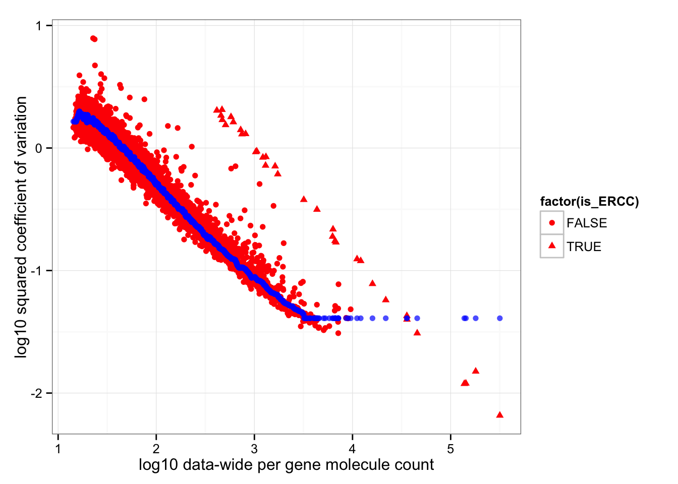
Compute adjusted coefficient of variation.
# adjusted coefficient of variation on log10 scale
log10cv2_adj <-
  lapply(1:length(molecules_cv_batch), function(per_batch) {
    foo <- log10(molecules_cv_batch[[per_batch]]$cv^2) - roll_medians
    return(foo)
})
df_plot$log10cv2_adj <- do.call(c, log10cv2_adj)
df_plot$is_ERCC <- ( 1:dim(df_plot)[1] %in% grep("ERCC", rownames(df_plot)) )
Adjusted squared coefficient of variation versus log10 mean count (CPM corrected).
ERCC remain the outliers after substracting out rolling medians.
ggplot( df_plot, aes(x = log10(mean), y = log10cv2_adj) ) +
  geom_point( aes(col = as.factor(batch), shape = factor(is_ERCC)), cex = .9 ) +
  facet_wrap( ~ batch) +
labs(x = "log10(Mean CPM)", y = "log10(Adjusted Squared coefficient of variation") 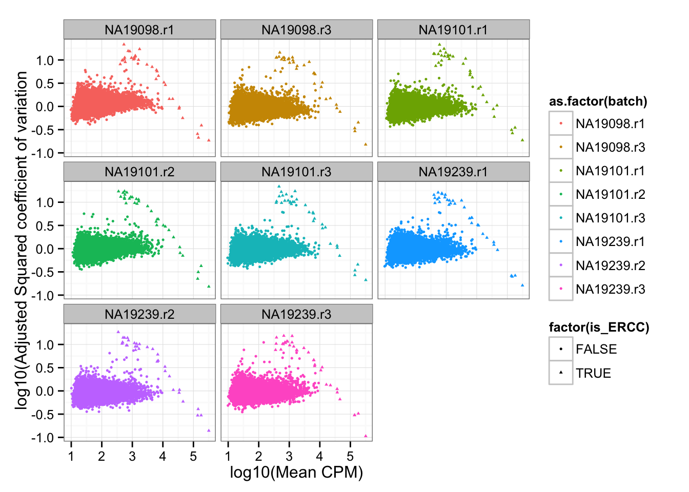
All genes: coefficient of variation after adjustment.
ggplot(df_plot, aes(x= factor(batch), y = log10cv2_adj, fill = factor(batch) ) ) +
  geom_violin(alpha = .5) +
  geom_boxplot(alpha = .01, width = .2, position = position_dodge(width = .9)) +
  labs(xlab = "log10 adjusted Squared coefficient of variation") +
  ggtitle( "log10 CV^2 after adjustment" )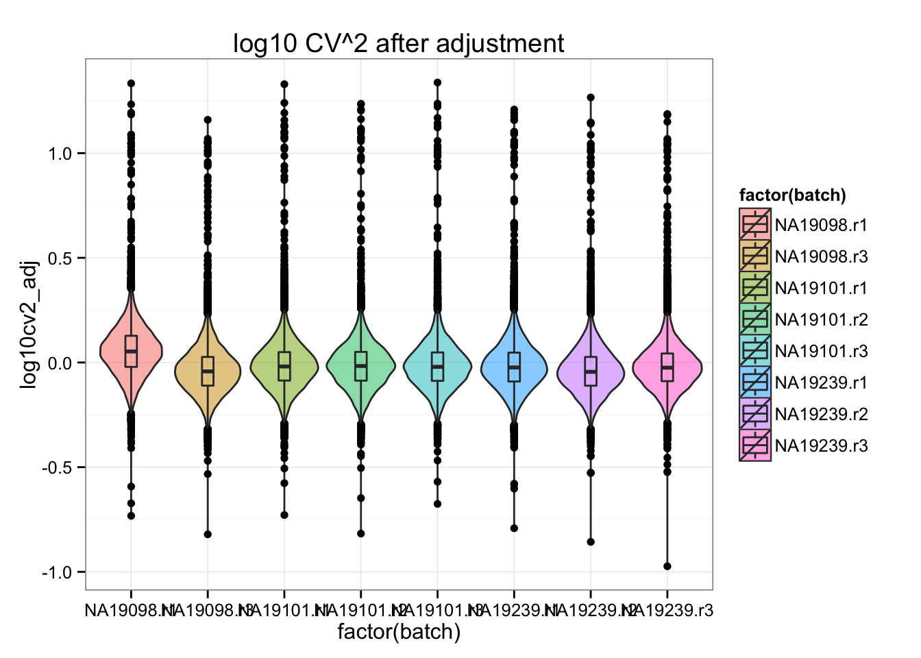
theme(axis.text.x = element_text(hjust=1, angle = 45))List of 1
$ axis.text.x:List of 8
..$ family : NULL
..$ face : NULL
..$ colour : NULL
..$ size : NULL
..$ hjust : num 1
..$ vjust : NULL
..$ angle : num 45
..$ lineheight: NULL
..- attr(*, "class")= chr [1:2] "element_text" "element"
- attr(*, "class")= chr [1:2] "theme" "gg"
- attr(*, "complete")= logi FALSEAll genes: coefficient of variation before adjustment.
ggplot(df_plot, aes(x= factor(batch), y = log10(cv^2), fill = factor(batch) ) ) +
  geom_violin(alpha = .5) +
  geom_boxplot(alpha = .01, width = .2, position = position_dodge(width = .9)) +
  labs(xlab = "log10 unadjusted Squared coefficient of variation") +
  ggtitle( "log10 CV^2 before adjustment" )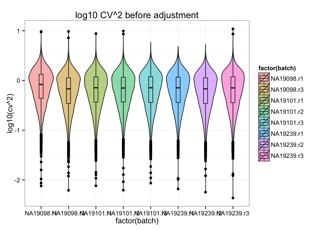
theme(axis.text.x = element_text(hjust=1, angle = 45))List of 1
$ axis.text.x:List of 8
..$ family : NULL
..$ face : NULL
..$ colour : NULL
..$ size : NULL
..$ hjust : num 1
..$ vjust : NULL
..$ angle : num 45
..$ lineheight: NULL
..- attr(*, "class")= chr [1:2] "element_text" "element"
- attr(*, "class")= chr [1:2] "theme" "gg"
- attr(*, "complete")= logi FALSEEndogeneous genes: coefficient of variation after adjustment.
ggplot(df_plot[which(!df_plot$is_ERCC), ], aes(x= factor(batch), y = log10cv2_adj, fill = factor(batch) ) ) +
  geom_violin(alpha = .5) +
  geom_boxplot(alpha = .01, width = .2, position = position_dodge(width = .9)) +
  labs(xlab = "log10 adjusted Squared coefficient of variation") +
  ggtitle( "log10 CV^2 after adjustment w/o ERCC" )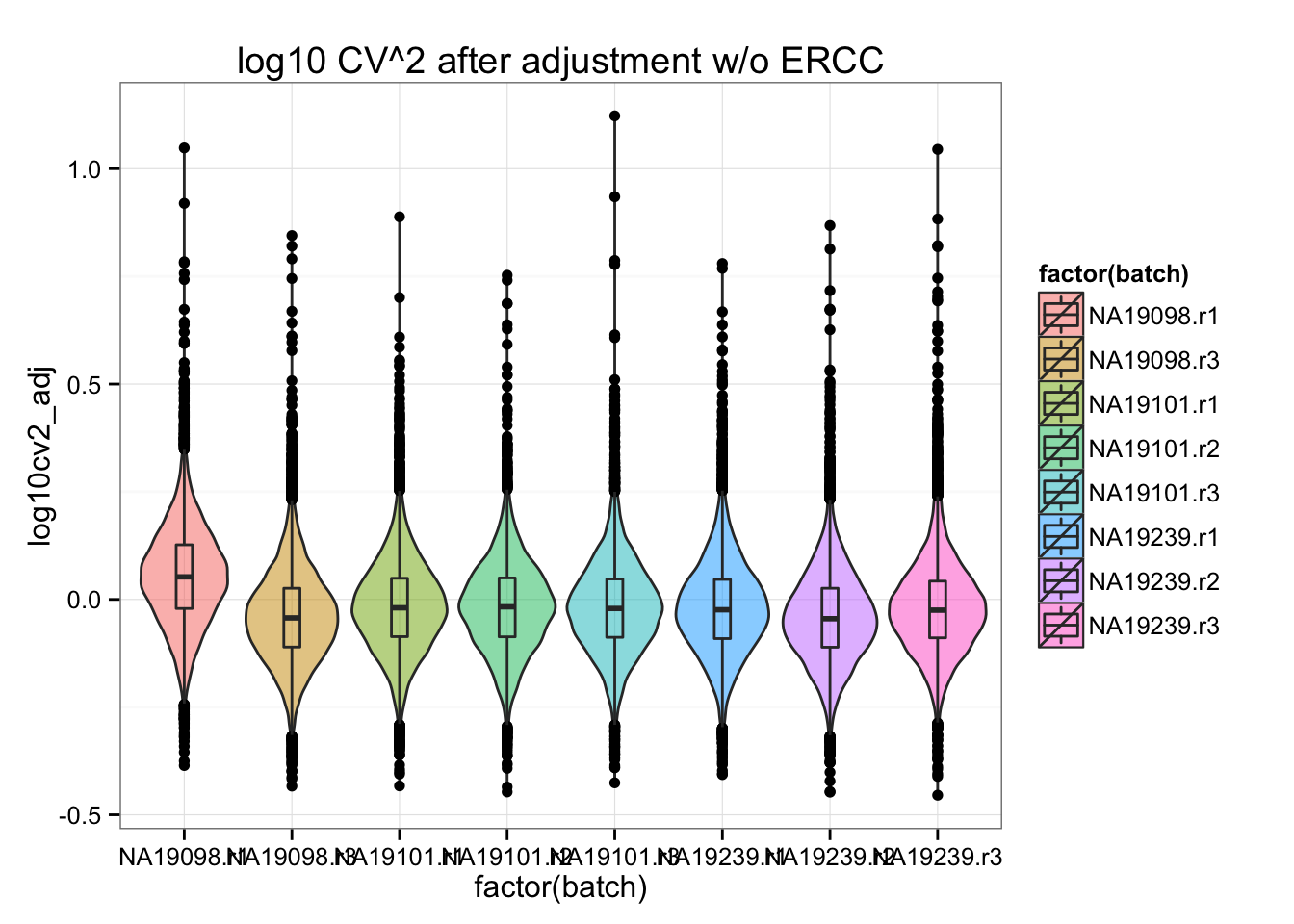
theme(axis.text.x = element_text(hjust=1, angle = 45))List of 1
$ axis.text.x:List of 8
..$ family : NULL
..$ face : NULL
..$ colour : NULL
..$ size : NULL
..$ hjust : num 1
..$ vjust : NULL
..$ angle : num 45
..$ lineheight: NULL
..- attr(*, "class")= chr [1:2] "element_text" "element"
- attr(*, "class")= chr [1:2] "theme" "gg"
- attr(*, "complete")= logi FALSEEndogeneous genes: coefficient of variation before adjustment.
ggplot(df_plot[which(!df_plot$is_ERCC), ], aes(x= factor(batch), y = log10(cv^2), fill = factor(batch) ) ) +
  geom_violin(alpha = .5) +
  geom_boxplot(alpha = .01, width = .2, position = position_dodge(width = .9)) +
  labs(xlab = "log10 unadjusted Squared coefficient of variation") +
  ggtitle( "log10 CV^2 before adjustment w/o ERCC" )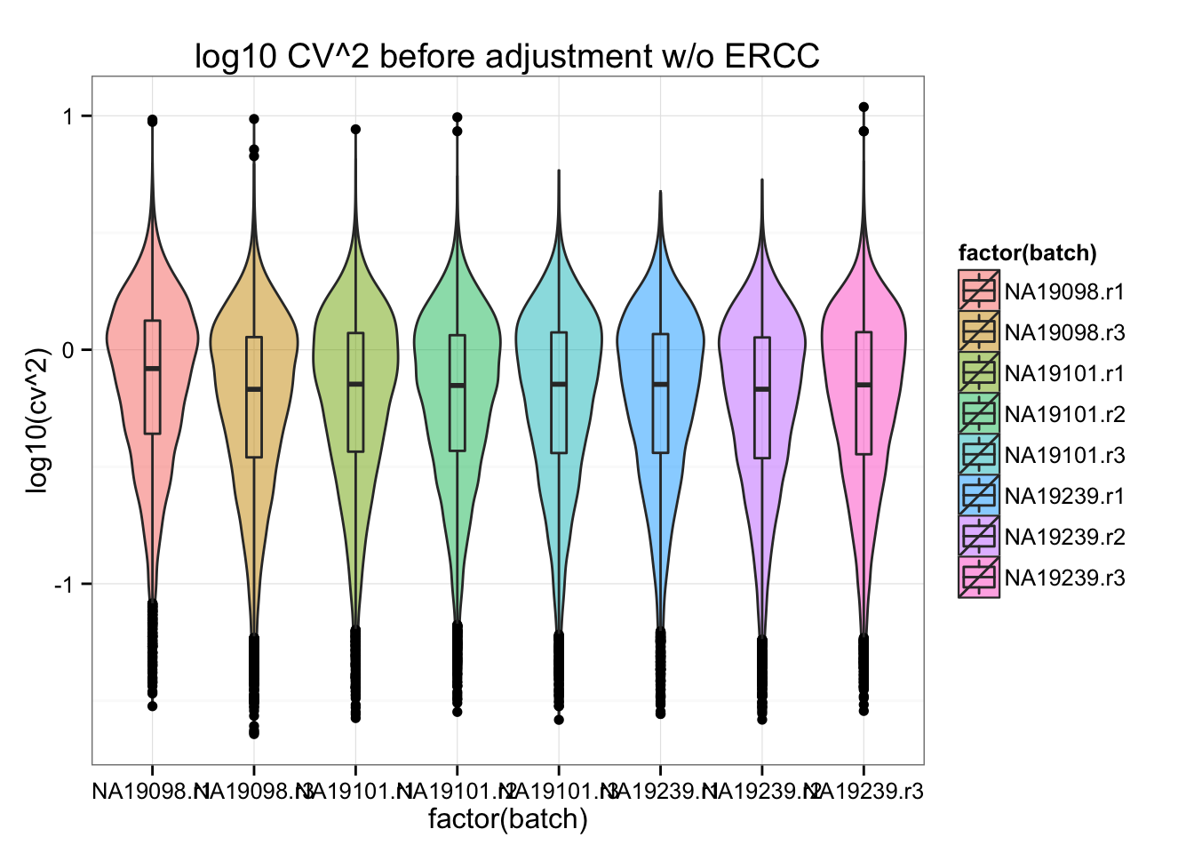
theme(axis.text.x = element_text(hjust=1, angle = 45))List of 1
$ axis.text.x:List of 8
..$ family : NULL
..$ face : NULL
..$ colour : NULL
..$ size : NULL
..$ hjust : num 1
..$ vjust : NULL
..$ angle : num 45
..$ lineheight: NULL
..- attr(*, "class")= chr [1:2] "element_text" "element"
- attr(*, "class")= chr [1:2] "theme" "gg"
- attr(*, "complete")= logi FALSESession information
sessionInfo()R version 3.2.1 (2015-06-18)
Platform: x86_64-apple-darwin13.4.0 (64-bit)
Running under: OS X 10.10.5 (Yosemite)
locale:
[1] en_US.UTF-8/en_US.UTF-8/en_US.UTF-8/C/en_US.UTF-8/en_US.UTF-8
attached base packages:
[1] grid stats graphics grDevices utils datasets methods
[8] base
other attached packages:
[1] zoo_1.7-12 ggplot2_1.0.1 edgeR_3.10.5 limma_3.24.15
[5] dplyr_0.4.3 data.table_1.9.6 knitr_1.11
loaded via a namespace (and not attached):
[1] Rcpp_0.12.2 magrittr_1.5 MASS_7.3-45 munsell_0.4.2
[5] lattice_0.20-33 colorspace_1.2-6 R6_2.1.1 stringr_1.0.0
[9] plyr_1.8.3 tools_3.2.1 parallel_3.2.1 gtable_0.1.2
[13] DBI_0.3.1 htmltools_0.2.6 yaml_2.1.13 assertthat_0.1
[17] digest_0.6.8 reshape2_1.4.1 formatR_1.2.1 evaluate_0.8
[21] rmarkdown_0.8.1 labeling_0.3 stringi_1.0-1 scales_0.3.0
[25] chron_2.3-47 proto_0.3-10