ERCC normalization
2015-06-15
- Setup
- Prepare single cell molecule data
- Prepare bulk cell read data
- Prepare ERCC data
- Raw non-normalized data
- Linear shift normalization
- RUVg normalization - k = 1
- RUVg with ERCC + invariant genes
- RUVg normalization - k = 3
- RUVg normalization - k = 9
- Empirical quantile normalization
- Loess normalization
- Session information
Last updated: 2015-09-21
Code version: 5ebd0cb11c559b6dd5b271dff713c64be62ac63b
Testing different approaches to normalize the data.
For the bulk samples, the data used is the TMM-normalized log2 reads per million. The only exception to this is with RUVg because it expects count data.
For the single cell samples, the data is the log2 molecules per million after correcting for the collision probability. The only exception to this is with RUVg because it expects count data. Also, batch 2 of individual 19098 is removed because its ERCC data is an outlier.
PCA is used to compare the results of the different normalizations. These calculations exclude the ERCC controls.
Setup
library("edgeR")
library("ggplot2")
theme_set(theme_bw(base_size = 16))
library("RUVSeq")
library("preprocessCore")
library("affy")
source("functions.R")
Input annotation.
anno <- read.table("../data/annotation.txt", header = TRUE,
                   stringsAsFactors = FALSE)
head(anno)
individual batch well sample_id
1 19098 1 A01 NA19098.1.A01
2 19098 1 A02 NA19098.1.A02
3 19098 1 A03 NA19098.1.A03
4 19098 1 A04 NA19098.1.A04
5 19098 1 A05 NA19098.1.A05
6 19098 1 A06 NA19098.1.A06Input read counts.
reads <- read.table("../data/reads.txt", header = TRUE,
                    stringsAsFactors = FALSE)
Input molecule counts.
molecules <- read.table("../data/molecules.txt", header = TRUE,
                    stringsAsFactors = FALSE)
Input ERCC concentration information.
ercc <- read.table("../data/ercc-info.txt", header = TRUE, sep = "\t",
                   stringsAsFactors = FALSE)
colnames(ercc) <- c("num", "id", "subgroup", "conc_mix1", "conc_mix2",
                    "expected_fc", "log2_mix1_mix2")
head(ercc)
num id subgroup conc_mix1 conc_mix2 expected_fc log2_mix1_mix2
1 1 ERCC-00130 A 30000.000 7500.00000 4 2
2 2 ERCC-00004 A 7500.000 1875.00000 4 2
3 3 ERCC-00136 A 1875.000 468.75000 4 2
4 4 ERCC-00108 A 937.500 234.37500 4 2
5 5 ERCC-00116 A 468.750 117.18750 4 2
6 6 ERCC-00092 A 234.375 58.59375 4 2stopifnot(nrow(ercc) == 92)Input list of quality single cells.
quality_single_cells <- scan("../data/quality-single-cells.txt",
                             what = "character")
Prepare single cell molecule data
Keep only the single cells that passed the QC filters. This also removes the bulk samples.
molecules_single <- molecules[, colnames(molecules) %in% quality_single_cells]
anno_single <- anno[anno$sample_id %in% quality_single_cells, ]
stopifnot(ncol(molecules_single) == nrow(anno_single),
          colnames(molecules_single) == anno_single$sample_id)
Also remove batch 2 of individual 19098.
molecules_single <- molecules_single[, !(anno_single$individual == 19098 & anno_single$batch == 2)]
anno_single <- anno_single[!(anno_single$individual == 19098 & anno_single$batch == 2), ]
stopifnot(ncol(molecules_single) == nrow(anno_single))
Remove genes with zero read counts in the single cells.
expressed_single <- rowSums(molecules_single) > 0
molecules_single <- molecules_single[expressed_single, ]
dim(molecules_single)
[1] 17478 563How many genes have greater than or equal to 1,024 molecules in at least one of the cells?
overexpressed_genes <- rownames(molecules_single)[apply(molecules_single, 1,
                                                        function(x) any(x >= 1024))]
15 have greater than or equal to 1,024 molecules. Remove them.
molecules_single <- molecules_single[!(rownames(molecules_single) %in% overexpressed_genes), ]Correct for the collision probability. See Grun et al. 2014 for details.
molecules_single_collision <- -1024 * log(1 - molecules_single / 1024)Standardize the molecule counts to account for differences in sequencing depth. This is necessary because the sequencing depth affects the total molecule counts.
molecules_single_cpm <- cpm(molecules_single_collision, log = TRUE)Prepare bulk cell read data
Select bulk samples.
reads_bulk <- reads[, anno$well == "bulk"]
anno_bulk <- anno[anno$well == "bulk", ]
stopifnot(ncol(reads_bulk) == nrow(anno_bulk),
          colnames(reads_bulk) == anno_bulk$sample_id)
Remove genes with zero reads in the bulk cells.
expressed_bulk <- rowSums(reads_bulk) > 0
reads_bulk <- reads_bulk[expressed_bulk, ]
dim(reads_bulk)
[1] 18123 9Calculate TMM-normalized read counts per million.
norm_factors_bulk <- calcNormFactors(reads_bulk, method = "TMM")
reads_bulk_cpm <- cpm(reads_bulk, log = TRUE,
                          lib.size = colSums(reads_bulk) * norm_factors_bulk)
Prepare ERCC data
Obtain the row indices for the ERCC spike-ins and the genes.
ercc_rows_single <- grep("ERCC", rownames(molecules_single))
gene_rows_single <- grep("ERCC", rownames(molecules_single), invert = TRUE)
ercc_rows_bulk <- grep("ERCC", rownames(reads_bulk))
gene_rows_bulk <- grep("ERCC", rownames(reads_bulk), invert = TRUE)
The single molecule data has 81 ERCC spike-ins and 17382 genes.
The bulk read data has 70 ERCC spike-ins and 18053 genes.
Sort ERCC data file by the spike-in ID.
ercc <- ercc[order(ercc$id), ]
# Also remove spike-ins with no counts
ercc_single <- ercc[ercc$id %in% rownames(molecules_single), ]
stopifnot(rownames(molecules_single[ercc_rows_single, ]) == ercc_single$id)
ercc_bulk <- ercc[ercc$id %in% rownames(reads_bulk), ]
stopifnot(rownames(reads_bulk[ercc_rows_bulk, ]) == ercc_bulk$id)
Raw non-normalized data
bulk log2 reads per million
pca_bulk_raw <- run_pca(reads_bulk_cpm[gene_rows_bulk, ])
plot_pca(pca_bulk_raw$PCs, explained = pca_bulk_raw$explained,
         metadata = anno_bulk, color = "individual",
         shape = "batch", factors = c("individual", "batch"))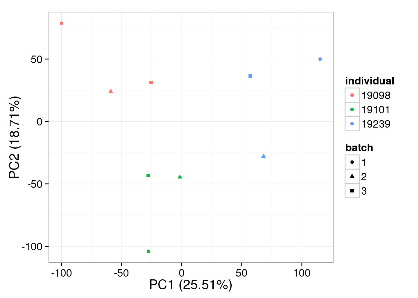
single log2 molecules per million
pca_single_raw <- run_pca(molecules_single_cpm[gene_rows_single, ])
plot_pca(pca_single_raw$PCs, explained = pca_single_raw$explained,
         metadata = anno_single, color = "individual",
         shape = "batch", factors = c("individual", "batch"))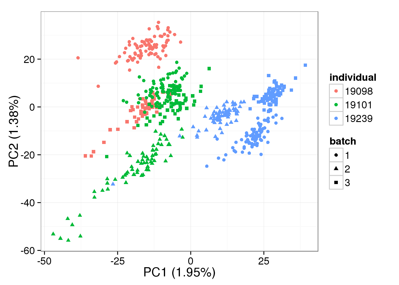
Linear shift normalization
Perform the normalization separately for bulk and single cells. Use the counts per million.
Adjust each individual sample based on its ERCC counts.
bulk_norm <- reads_bulk_cpm
bulk_norm[, ] <- NA
for (i in 1:ncol(bulk_norm)) {
  bulk_fit <- lm(reads_bulk_cpm[ercc_rows_bulk, i] ~ log2(ercc_bulk$conc_mix1))
  # Y = mX + b -> X = (Y + b) / m
  bulk_norm[, i] <- (reads_bulk_cpm[, i] + bulk_fit$coefficients[1]) /
                     bulk_fit$coefficients[2]
}
stopifnot(!is.na(bulk_norm))
single_norm <- molecules_single_cpm
single_norm[, ] <- NA
for (i in 1:ncol(single_norm)) {
single_fit <- lm(molecules_single_cpm[ercc_rows_single, i] ~ log2(ercc_single$conc_mix1))
# Y = mX + b -> X = (Y - b) / m
single_norm[, i] <- (molecules_single_cpm[, i] - single_fit$coefficients[1]) /
single_fit$coefficients[2]
}
stopifnot(!is.na(single_norm))bulk log2 reads per million
pca_bulk_norm <- run_pca(bulk_norm[gene_rows_bulk, ])
plot_pca(pca_bulk_norm$PCs, explained = pca_bulk_norm$explained,
         metadata = anno_bulk, color = "individual",
         shape = "batch", factors = c("individual", "batch"))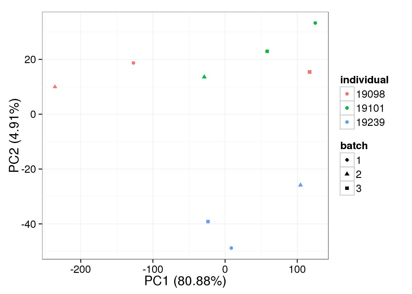
single log2 molecules per million
pca_single_norm <- run_pca(single_norm[gene_rows_single, ])
plot_pca(pca_single_norm$PCs, explained = pca_single_norm$explained,
         metadata = anno_single, color = "individual",
         shape = "batch", factors = c("individual", "batch"))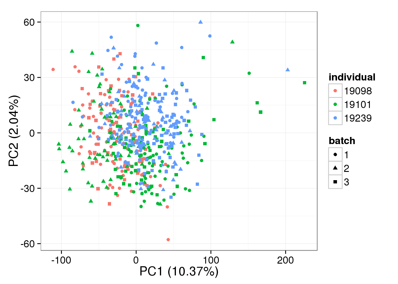
RUVg normalization - k = 1
Use RUVg from Risso et al., 2014. It uses the ERCC spike-ins as negative control genes to correct for unwanted variation. It uses counts as input and output. It requires one parameter to be chosen: k is the “number of factors of unwanted variation to be estimated from the data”.
For k = 1:
bulk_ruv_object_k1 <- RUVg(x = as.matrix(reads_bulk), cIdx = ercc_rows_bulk, k = 1)
bulk_ruv_k1 <- bulk_ruv_object_k1$normalizedCounts
bulk_ruv_cpm_k1 <- cpm(bulk_ruv_k1, log = TRUE,
                       lib.size = calcNormFactors(bulk_ruv_k1) * colSums(bulk_ruv_k1))
single_ruv_object_k1 <- RUVg(x = as.matrix(molecules_single), cIdx = ercc_rows_single, k = 1)
single_ruv_k1 <- single_ruv_object_k1$normalizedCounts
single_ruv_cpm_k1 <- cpm(single_ruv_k1, log = TRUE,
lib.size = calcNormFactors(single_ruv_k1) * colSums(single_ruv_k1))bulk log2 reads per million
pca_bulk_ruv_k1 <- run_pca(bulk_ruv_cpm_k1[gene_rows_bulk, ])
plot_pca(pca_bulk_ruv_k1$PCs, explained = pca_bulk_ruv_k1$explained,
         metadata = anno_bulk, color = "individual",
         shape = "batch", factors = c("individual", "batch"))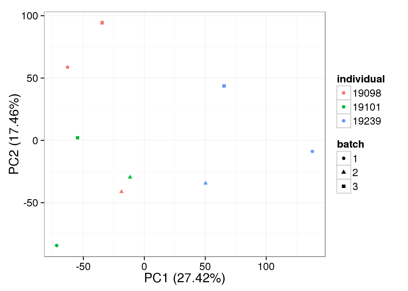
single log2 molecules per million
pca_single_ruv_k1 <- run_pca(single_ruv_cpm_k1[gene_rows_single, ])
plot_pca(pca_single_ruv_k1$PCs, explained = pca_single_ruv_k1$explained,
         metadata = anno_single, color = "individual",
         shape = "batch", factors = c("individual", "batch"))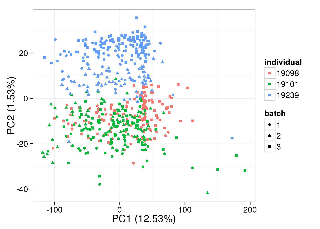
RUVg with ERCC + invariant genes
As an attempt to improve performance of RUVg, also include invariant genes. The genes were chosen using the following procedure:
- Require the genes are observed in at least half the cells.
- Exclude ERCC genes.
- Choose the 10% with the lowest variance (using the counts standardized by total depth).
First for the bulk cells:
bulk_variance <- apply(reads_bulk_cpm, 1, var)
summary(bulk_variance)
Min. 1st Qu. Median Mean 3rd Qu. Max.
0.00198 0.04364 0.13150 0.79320 0.76500 21.85000 sum(bulk_variance == 0)[1] 0names(bulk_variance) <- rownames(reads_bulk_cpm)
# Require that the genes are observed in at least half the cells
bulk_variance <- bulk_variance[apply(reads_bulk, 1,
function(x) {sum(x > 0) >= length(x) * 0.5})]
# Remove ERCC genes
bulk_variance <- bulk_variance[grep("ERCC", names(bulk_variance),
invert = TRUE)]
# Choose the bottom 10%
bulk_least_variant <- names(bulk_variance)[order(bulk_variance)][1:floor(length(bulk_variance) * .1)]
# Identify the rows
bulk_least_variant_rows <- which(rownames(reads_bulk_cpm) %in% bulk_least_variant)This procedure identified 1602 genes that have low variance and are observed in at least half of the bulk cells.
For k = 1:
bulk_ruv_object_invar_k1 <- RUVg(x = as.matrix(reads_bulk),
                                cIdx = c(ercc_rows_bulk, bulk_least_variant_rows),
                                k = 1)
bulk_ruv_invar_k1 <- bulk_ruv_object_invar_k1$normalizedCounts
bulk_ruv_cpm_invar_k1 <- cpm(bulk_ruv_invar_k1, log = TRUE,
                            lib.size = calcNormFactors(bulk_ruv_invar_k1) *
                                       colSums(bulk_ruv_invar_k1))
For k = 3:
bulk_ruv_object_invar_k3 <- RUVg(x = as.matrix(reads_bulk),
                                cIdx = c(ercc_rows_bulk, bulk_least_variant_rows),
                                k = 3)
bulk_ruv_invar_k3 <- bulk_ruv_object_invar_k3$normalizedCounts
bulk_ruv_cpm_invar_k3 <- cpm(bulk_ruv_invar_k3, log = TRUE,
                            lib.size = calcNormFactors(bulk_ruv_invar_k3) *
                                       colSums(bulk_ruv_invar_k3))
Second for the single cells:
single_variance <- apply(molecules_single_cpm, 1, var)
summary(single_variance)
Min. 1st Qu. Median Mean 3rd Qu. Max.
0.004061 0.285100 1.134000 1.277000 2.257000 10.320000 sum(single_variance == 0)[1] 0names(single_variance) <- rownames(molecules_single_cpm)
# Require that the genes are observed in at least half the cells
single_variance <- single_variance[apply(molecules_single, 1,
function(x) {sum(x > 0) >= length(x) * 0.5})]
# Remove ERCC genes
single_variance <- single_variance[grep("ERCC", names(single_variance),
invert = TRUE)]
# Choose the bottom 10%
single_least_variant <- names(single_variance)[order(single_variance)][1:floor(length(single_variance) * .1)]
# Identify the rows
single_least_variant_rows <- which(rownames(molecules_single_cpm) %in% single_least_variant)This procedure identified 875 genes that have low variance and are observed in at least half of the single cells.
For k = 1:
single_ruv_object_invar_k1 <- RUVg(x = as.matrix(molecules_single),
                                cIdx = c(ercc_rows_single, single_least_variant_rows),
                                k = 1)
single_ruv_invar_k1 <- single_ruv_object_invar_k1$normalizedCounts
single_ruv_cpm_invar_k1 <- cpm(single_ruv_invar_k1, log = TRUE,
                            lib.size = calcNormFactors(single_ruv_invar_k1) *
                                       colSums(single_ruv_invar_k1))
For k = 3:
single_ruv_object_invar_k3 <- RUVg(x = as.matrix(molecules_single),
                                cIdx = c(ercc_rows_single, single_least_variant_rows),
                                k = 3)
single_ruv_invar_k3 <- single_ruv_object_invar_k3$normalizedCounts
single_ruv_cpm_invar_k3 <- cpm(single_ruv_invar_k3, log = TRUE,
                            lib.size = calcNormFactors(single_ruv_invar_k3) *
                                       colSums(single_ruv_invar_k3))
For k = 9:
single_ruv_object_invar_k9 <- RUVg(x = as.matrix(molecules_single),
                                cIdx = c(ercc_rows_single, single_least_variant_rows),
                                k = 9)
single_ruv_invar_k9 <- single_ruv_object_invar_k9$normalizedCounts
single_ruv_cpm_invar_k9 <- cpm(single_ruv_invar_k9, log = TRUE,
                            lib.size = calcNormFactors(single_ruv_invar_k9) *
                                       colSums(single_ruv_invar_k9))
For k = 30:
single_ruv_object_invar_k30 <- RUVg(x = as.matrix(molecules_single),
                                cIdx = c(ercc_rows_single, single_least_variant_rows),
                                k = 30)
single_ruv_invar_k30 <- single_ruv_object_invar_k30$normalizedCounts
single_ruv_cpm_invar_k30 <- cpm(single_ruv_invar_k30, log = TRUE,
                            lib.size = calcNormFactors(single_ruv_invar_k30) *
                                       colSums(single_ruv_invar_k30))
bulk log2 reads per million - k = 1
pca_bulk_ruv_invar_k1 <- run_pca(bulk_ruv_cpm_invar_k1[gene_rows_bulk, ])
plot_pca(pca_bulk_ruv_invar_k1$PCs, explained = pca_bulk_ruv_invar_k1$explained,
         metadata = anno_bulk, color = "individual",
         shape = "batch", factors = c("individual", "batch"))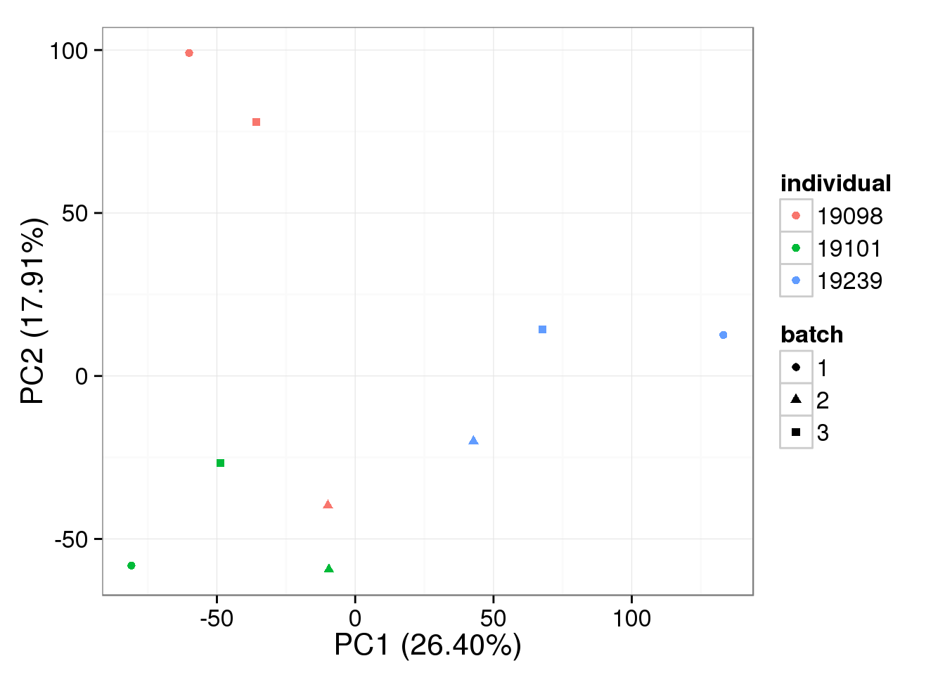
bulk log2 reads per million - k = 3
pca_bulk_ruv_invar_k3 <- run_pca(bulk_ruv_cpm_invar_k3[gene_rows_bulk, ])
plot_pca(pca_bulk_ruv_invar_k3$PCs, explained = pca_bulk_ruv_invar_k3$explained,
         metadata = anno_bulk, color = "individual",
         shape = "batch", factors = c("individual", "batch"))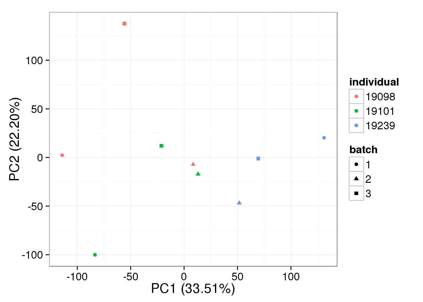
single log2 molecules per million - k = 1
pca_single_ruv_invar_k1 <- run_pca(single_ruv_cpm_invar_k1[gene_rows_single, ])
plot_pca(pca_single_ruv_invar_k1$PCs, explained = pca_single_ruv_invar_k1$explained,
         metadata = anno_single, color = "individual",
         shape = "batch", factors = c("individual", "batch"))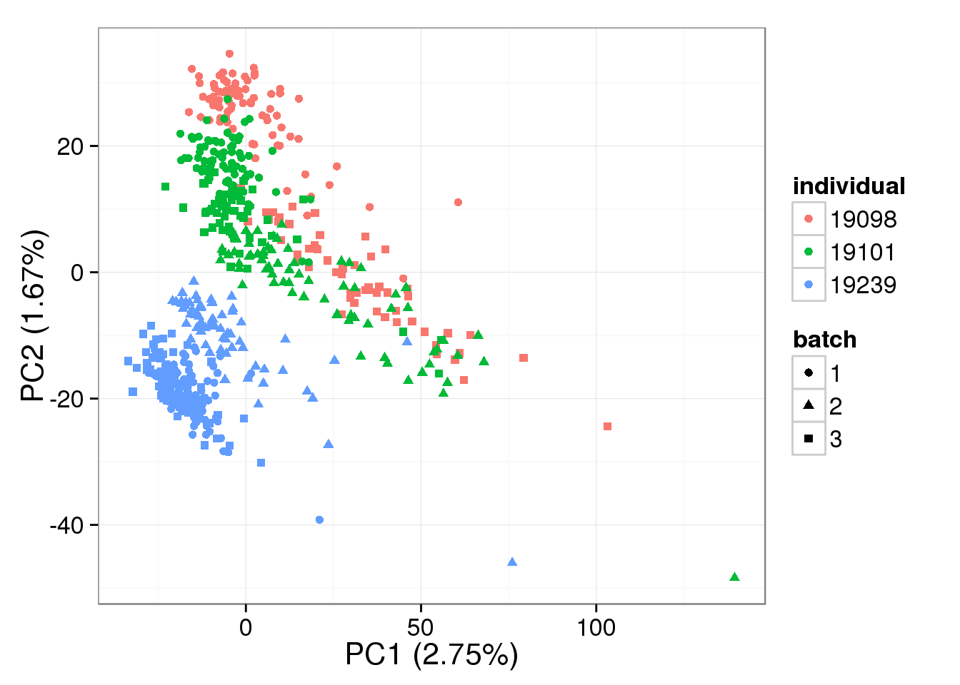
single log2 molecules per million - k = 3
pca_single_ruv_invar_k3 <- run_pca(single_ruv_cpm_invar_k3[gene_rows_single, ])
plot_pca(pca_single_ruv_invar_k3$PCs, explained = pca_single_ruv_invar_k3$explained,
         metadata = anno_single, color = "individual",
         shape = "batch", factors = c("individual", "batch"))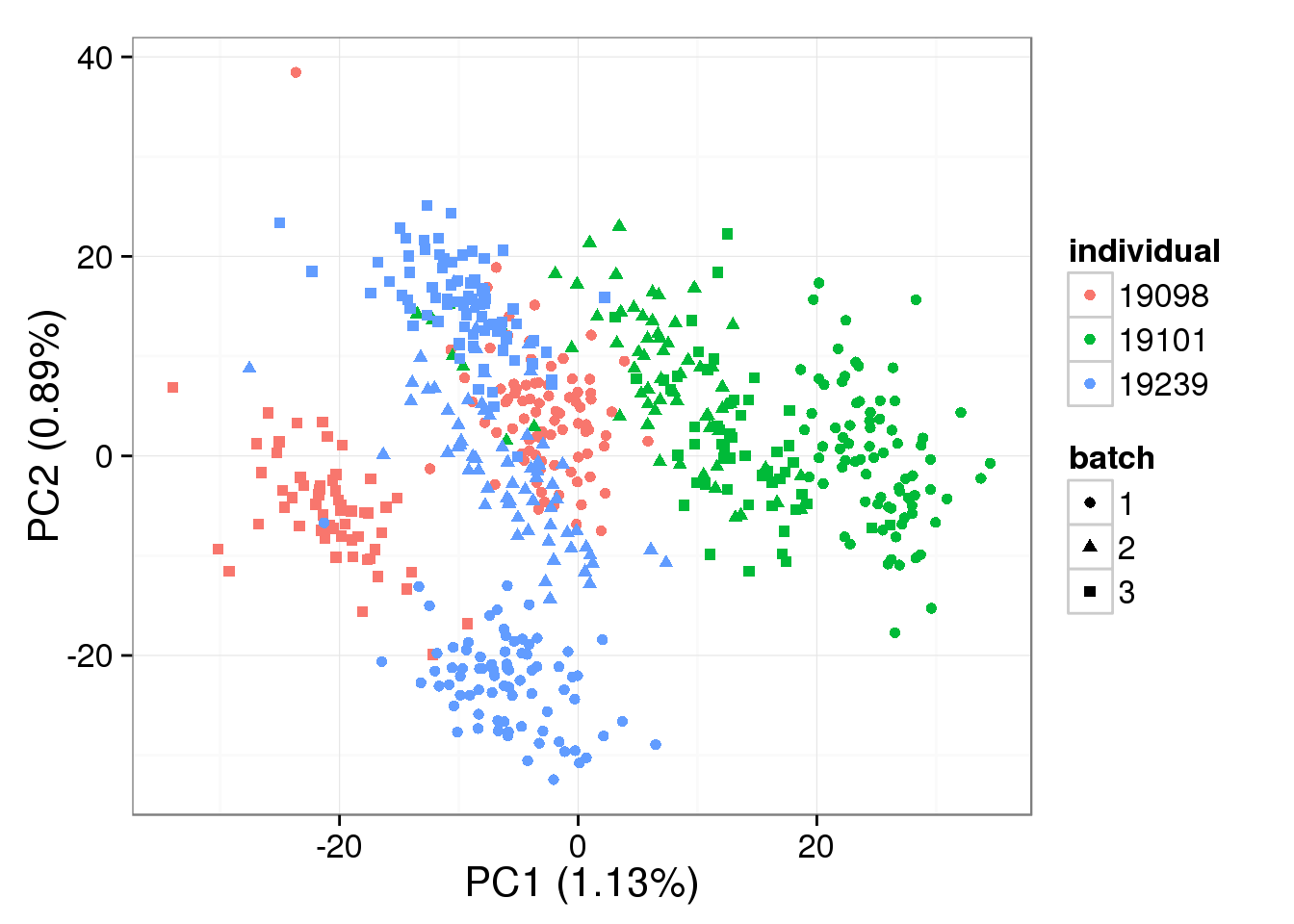
single log2 molecules per million - k = 9
pca_single_ruv_invar_k9 <- run_pca(single_ruv_cpm_invar_k9[gene_rows_single, ])
plot_pca(pca_single_ruv_invar_k9$PCs, explained = pca_single_ruv_invar_k9$explained,
         metadata = anno_single, color = "individual",
         shape = "batch", factors = c("individual", "batch"))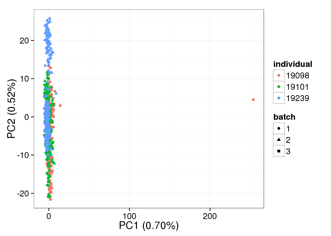
single log2 molecules per million - k = 30
pca_single_ruv_invar_k30 <- run_pca(single_ruv_cpm_invar_k30[gene_rows_single, ])
plot_pca(pca_single_ruv_invar_k30$PCs, explained = pca_single_ruv_invar_k30$explained,
         metadata = anno_single, color = "individual",
         shape = "batch", factors = c("individual", "batch"))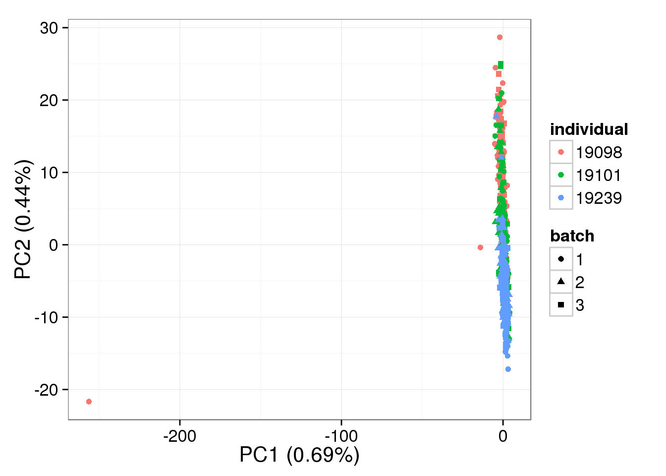
RUVg normalization - k = 3
bulk_ruv_object_k3 <- RUVg(x = as.matrix(reads_bulk), cIdx = ercc_rows_bulk, k = 3)
bulk_ruv_k3 <- bulk_ruv_object_k3$normalizedCounts
bulk_ruv_cpm_k3 <- cpm(bulk_ruv_k3, log = TRUE,
                       lib.size = calcNormFactors(bulk_ruv_k3) * colSums(bulk_ruv_k3))
single_ruv_object_k3 <- RUVg(x = as.matrix(molecules_single), cIdx = ercc_rows_single, k = 3)
single_ruv_k3 <- single_ruv_object_k3$normalizedCounts
single_ruv_cpm_k3 <- cpm(single_ruv_k3, log = TRUE,
lib.size = calcNormFactors(single_ruv_k3) * colSums(single_ruv_k3))bulk log2 reads per million
RUVg-normalized bulk data with k = 3:
pca_bulk_ruv_k3 <- run_pca(bulk_ruv_cpm_k3[gene_rows_bulk, ])
plot_pca(pca_bulk_ruv_k3$PCs, explained = pca_bulk_ruv_k3$explained,
         metadata = anno_bulk, color = "individual",
         shape = "batch", factors = c("individual", "batch"))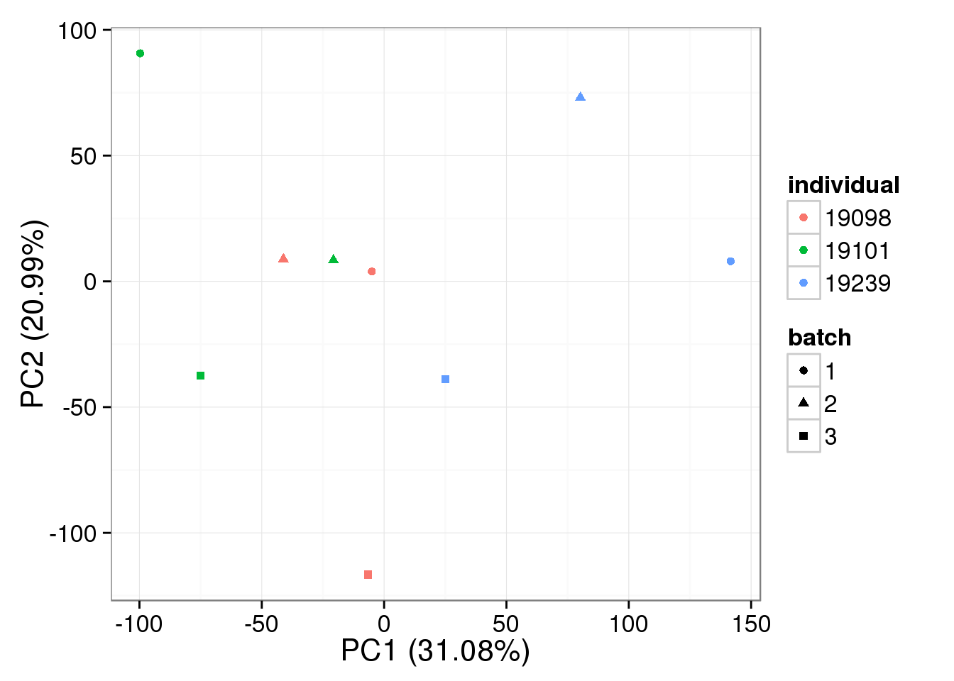
single log2 molecules per million
RUVg-normalized single cell data with k = 3:
pca_single_ruv_k3 <- run_pca(single_ruv_cpm_k3[gene_rows_single, ])
plot_pca(pca_single_ruv_k3$PCs, explained = pca_single_ruv_k3$explained,
         metadata = anno_single, color = "individual",
         shape = "batch", factors = c("individual", "batch"))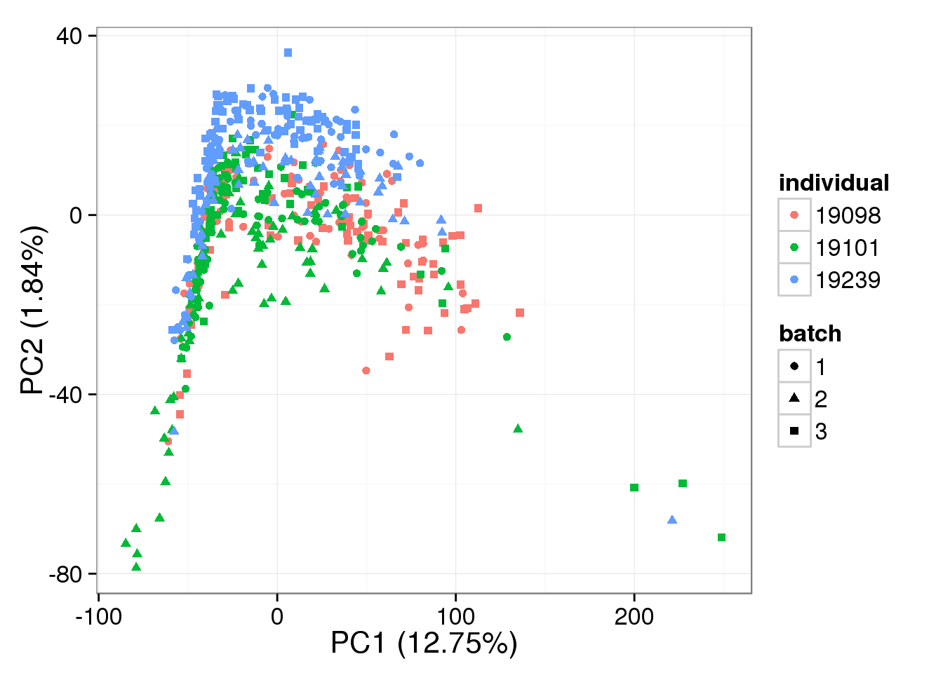
RUVg normalization - k = 9
bulk_ruv_object_k9 <- RUVg(x = as.matrix(reads_bulk), cIdx = ercc_rows_bulk, k = 9)
bulk_ruv_k9 <- bulk_ruv_object_k9$normalizedCounts
bulk_ruv_cpm_k9 <- cpm(bulk_ruv_k9, log = TRUE,
                       lib.size = calcNormFactors(bulk_ruv_k9) * colSums(bulk_ruv_k9))
single_ruv_object_k9 <- RUVg(x = as.matrix(molecules_single), cIdx = ercc_rows_single, k = 9)
single_ruv_k9 <- single_ruv_object_k9$normalizedCounts
single_ruv_cpm_k9 <- cpm(single_ruv_k9, log = TRUE,
lib.size = calcNormFactors(single_ruv_k9) * colSums(single_ruv_k9))bulk log2 reads per million
k = 9 removes all gene expression variation from the bulk data:
sum(apply(bulk_ruv_cpm_k9[gene_rows_bulk, ], 1, var) == 0)[1] 18053nrow(bulk_ruv_cpm_k9[gene_rows_bulk, ])[1] 18053single log2 molecules per million
RUVg-normalized single cell data with k = 9:
pca_single_ruv_k9 <- run_pca(single_ruv_cpm_k9[gene_rows_single, ])
plot_pca(pca_single_ruv_k9$PCs, explained = pca_single_ruv_k9$explained,
         metadata = anno_single, color = "individual",
         shape = "batch", factors = c("individual", "batch"))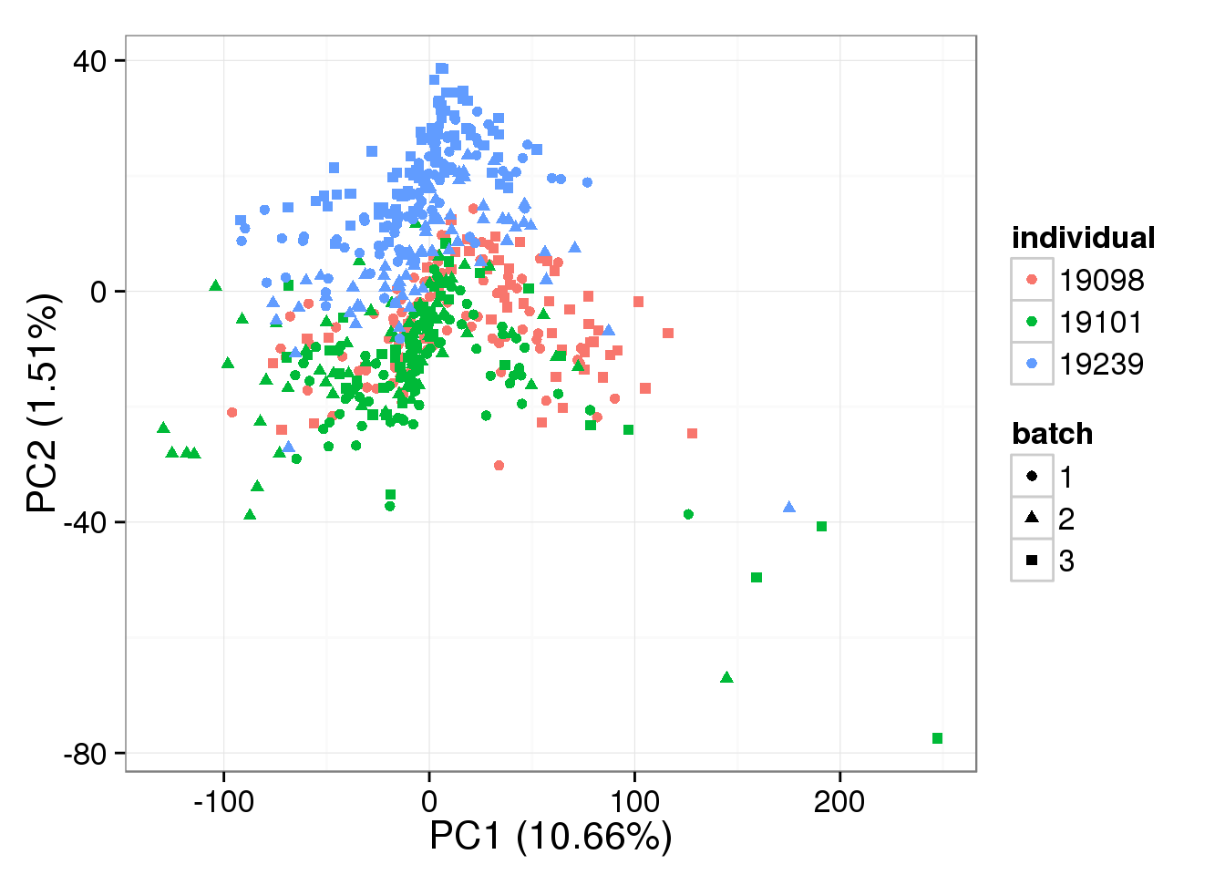
RUVg normalization - k = 30
For k = 30 for single cells only:
single_ruv_object_k30 <- RUVg(x = as.matrix(molecules_single), cIdx = ercc_rows_single, k = 30)
single_ruv_k30 <- single_ruv_object_k30$normalizedCounts
single_ruv_cpm_k30 <- cpm(single_ruv_k30, log = TRUE,
                      lib.size = calcNormFactors(single_ruv_k30) * colSums(single_ruv_k30))
single log2 molecules per million
pca_single_ruv_k30 <- run_pca(single_ruv_cpm_k30[gene_rows_single, ])
plot_pca(pca_single_ruv_k30$PCs, explained = pca_single_ruv_k30$explained,
         metadata = anno_single, color = "individual",
         shape = "batch", factors = c("individual", "batch"))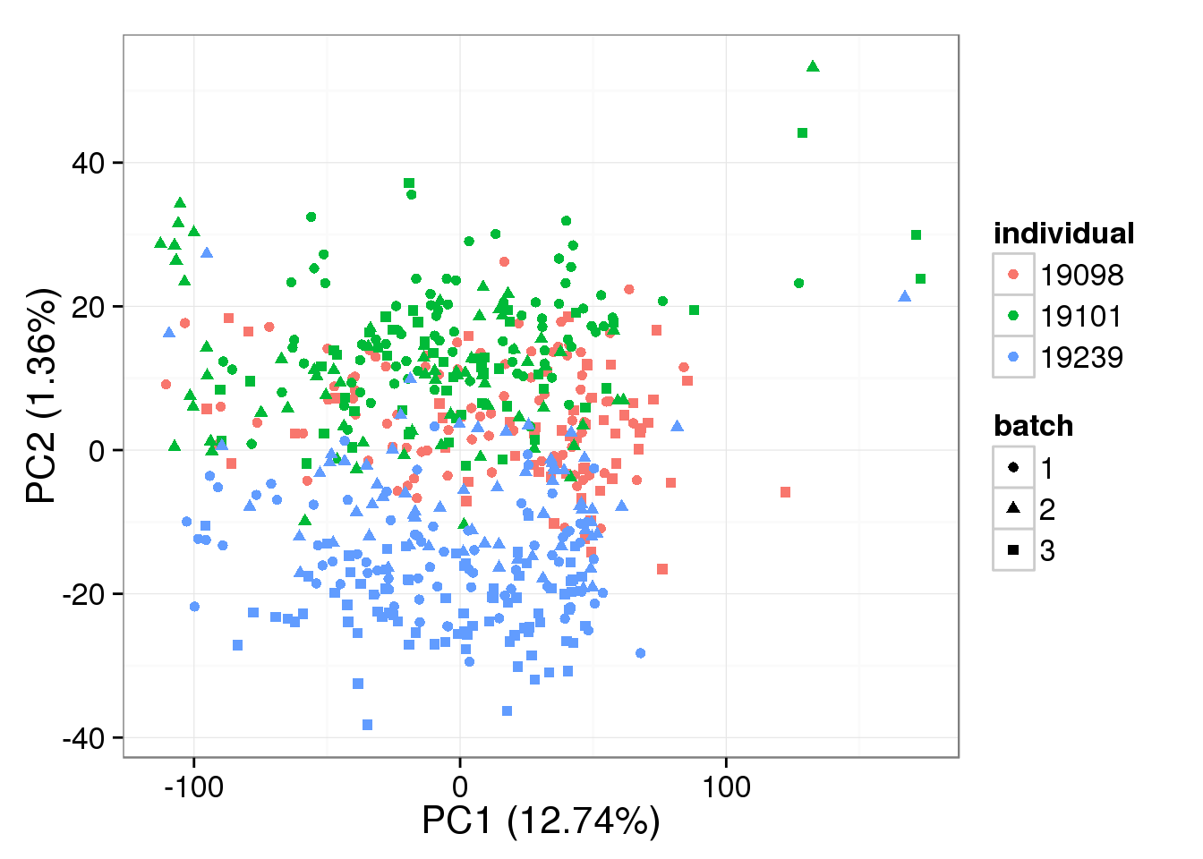
Empirical quantile normalization
Instead of using the ERCC specifically as a guide, simply perform an empirical quantile normalization (including both the genes and ERCC controls).
# from package preprocessCore
bulk_quant <- normalize.quantiles(as.matrix(reads_bulk_cpm))
single_quant <- normalize.quantiles(as.matrix(molecules_single_cpm))bulk log2 reads per million
pca_bulk_quant <- run_pca(bulk_quant[gene_rows_bulk, ])
plot_pca(pca_bulk_quant$PCs, explained = pca_bulk_quant$explained,
         metadata = anno_bulk, color = "individual",
         shape = "batch", factors = c("individual", "batch"))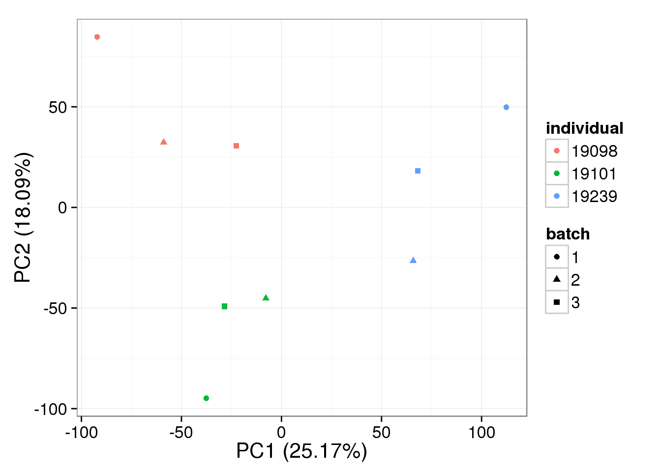
single log2 molecules per million
Quantile-normalized single cell data:
pca_single_quant <- run_pca(single_quant[gene_rows_single, ])
plot_pca(pca_single_quant$PCs, explained = pca_single_quant$explained,
         metadata = anno_single, color = "individual",
         shape = "batch", factors = c("individual", "batch"))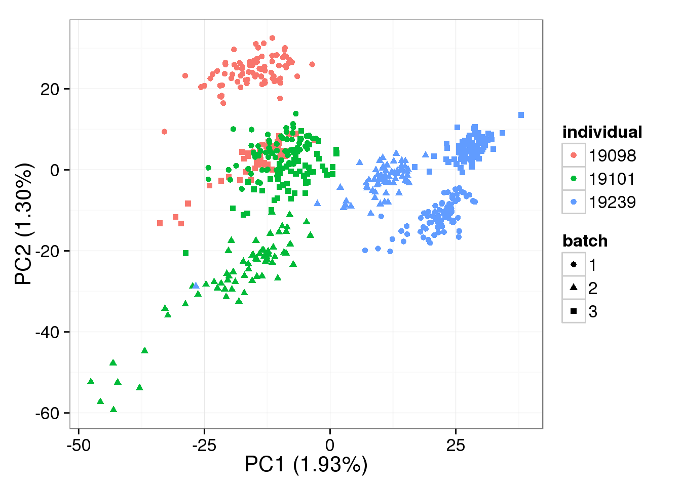
Loess normalization
Lovén et al. 2014 used a loess regression to normalize expression data with the ERCC probes. Below is their description:
We used a loess regression to renormalize these MAS5 normalized probe set values by using only the spike-in probe sets to fit the loess. The affy package provides a function, loess.normalize, which will perform loess regression on a matrix of values (defined by using the parameter mat) and allows for the user to specify which subset of data to use when fitting the loess (defined by using the parameter subset, see the affy package documentation for further details). For this application, the parameters mat and subset were set as the MAS5-normalized values and the row indices of the ERCC control probe sets, respectively. The default settings for all other parameters were used. The result of this was a matrix of expression values normalized to the control ERCC probes.
Risso et al. 2014 argue that regression-based approaches like this and the linear shift performed above do not work well:
The good performance of RUVg compared to global-scaling and regression-based normalization can be explained by the different assumptions underlying each approach. Global-scaling and regression-based normalization methods assume that unwanted technical effects (i.e., between-sample differences excluding biological effects of interest) are roughly the same for genes and spike-ins and are captured by either a single parameter per sample or a regression function between pairs of samples. Such assumptions were clearly violated for our data sets (e.g., Fig. 4d). RUVg, on the other hand, only assumes that the factors of unwanted variation estimated from the spike-ins span the same linear space as the factors of unwanted variation W for all of the genes.
# From the package affy
bulk_loess <- normalize.loess(mat = as.matrix(reads_bulk_cpm),
                              subset = ercc_rows_bulk, log.it = FALSE)
Done with 1 vs 2 in iteration 1
Done with 1 vs 3 in iteration 1
Done with 1 vs 4 in iteration 1
Done with 1 vs 5 in iteration 1
Done with 1 vs 6 in iteration 1
Done with 1 vs 7 in iteration 1
Done with 1 vs 8 in iteration 1
Done with 1 vs 9 in iteration 1
Done with 2 vs 3 in iteration 1
Done with 2 vs 4 in iteration 1
Done with 2 vs 5 in iteration 1
Done with 2 vs 6 in iteration 1
Done with 2 vs 7 in iteration 1
Done with 2 vs 8 in iteration 1
Done with 2 vs 9 in iteration 1
Done with 3 vs 4 in iteration 1
Done with 3 vs 5 in iteration 1
Done with 3 vs 6 in iteration 1
Done with 3 vs 7 in iteration 1
Done with 3 vs 8 in iteration 1
Done with 3 vs 9 in iteration 1
Done with 4 vs 5 in iteration 1
Done with 4 vs 6 in iteration 1
Done with 4 vs 7 in iteration 1
Done with 4 vs 8 in iteration 1
Done with 4 vs 9 in iteration 1
Done with 5 vs 6 in iteration 1
Done with 5 vs 7 in iteration 1
Done with 5 vs 8 in iteration 1
Done with 5 vs 9 in iteration 1
Done with 6 vs 7 in iteration 1
Done with 6 vs 8 in iteration 1
Done with 6 vs 9 in iteration 1
Done with 7 vs 8 in iteration 1
Done with 7 vs 9 in iteration 1
Done with 8 vs 9 in iteration 1
1 6.202689 There is an issue with the ercc controls when trying to perform loess regression. It appears fine when there is no subsetting, but it takes so long to run I didn’t let it finish. Since the loess regression on the bulk samples gives a similar to result to the linear shift (not surprisingly since they are both regression-based methods), this does not seem worth the effort to debug. The code below is a record of what I tried and is not evaluated.
single_loess <- normalize.loess(mat = as.matrix(molecules_single_cpm),
                                subset = ercc_rows_single, log.it = FALSE)
bulk log2 reads per million
Loess-normalized bulk data:
pca_bulk_loess <- run_pca(bulk_loess[gene_rows_bulk, ])
plot_pca(pca_bulk_loess$PCs, explained = pca_bulk_loess$explained,
         metadata = anno_bulk, color = "individual",
         shape = "batch", factors = c("individual", "batch"))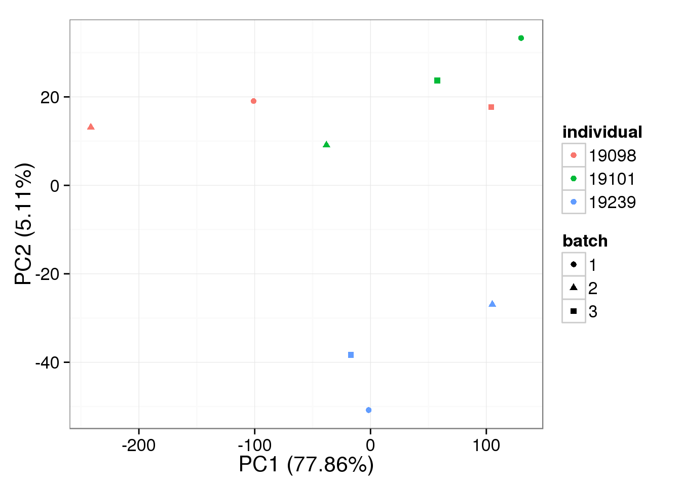
Session information
sessionInfo()R version 3.2.0 (2015-04-16)
Platform: x86_64-unknown-linux-gnu (64-bit)
locale:
[1] LC_CTYPE=en_US.UTF-8 LC_NUMERIC=C
[3] LC_TIME=en_US.UTF-8 LC_COLLATE=en_US.UTF-8
[5] LC_MONETARY=en_US.UTF-8 LC_MESSAGES=en_US.UTF-8
[7] LC_PAPER=en_US.UTF-8 LC_NAME=C
[9] LC_ADDRESS=C LC_TELEPHONE=C
[11] LC_MEASUREMENT=en_US.UTF-8 LC_IDENTIFICATION=C
attached base packages:
[1] stats4 parallel stats graphics grDevices utils datasets
[8] methods base
other attached packages:
[1] testit_0.4 affy_1.46.0
[3] preprocessCore_1.30.0 RUVSeq_1.2.0
[5] EDASeq_2.2.0 ShortRead_1.26.0
[7] GenomicAlignments_1.4.1 Rsamtools_1.20.4
[9] GenomicRanges_1.20.5 GenomeInfoDb_1.4.0
[11] Biostrings_2.36.1 XVector_0.8.0
[13] IRanges_2.2.4 S4Vectors_0.6.0
[15] BiocParallel_1.2.2 Biobase_2.28.0
[17] BiocGenerics_0.14.0 ggplot2_1.0.1
[19] edgeR_3.10.2 limma_3.24.9
[21] knitr_1.10.5
loaded via a namespace (and not attached):
[1] Rcpp_0.12.0 lattice_0.20-31 digest_0.6.8
[4] plyr_1.8.3 futile.options_1.0.0 aroma.light_2.4.0
[7] RSQLite_1.0.0 DESeq_1.20.0 evaluate_0.7
[10] BiocInstaller_1.18.4 zlibbioc_1.14.0 annotate_1.46.0
[13] R.utils_2.1.0 R.oo_1.19.0 rmarkdown_0.6.1
[16] proto_0.3-10 labeling_0.3 splines_3.2.0
[19] geneplotter_1.46.0 stringr_1.0.0 munsell_0.4.2
[22] htmltools_0.2.6 matrixStats_0.14.0 XML_3.98-1.2
[25] MASS_7.3-40 bitops_1.0-6 R.methodsS3_1.7.0
[28] grid_3.2.0 xtable_1.7-4 gtable_0.1.2
[31] DBI_0.3.1 magrittr_1.5 formatR_1.2
[34] scales_0.2.4 stringi_0.4-1 hwriter_1.3.2
[37] reshape2_1.4.1 genefilter_1.50.0 affyio_1.36.0
[40] latticeExtra_0.6-26 futile.logger_1.4.1 lambda.r_1.1.7
[43] RColorBrewer_1.1-2 tools_3.2.0 survival_2.38-1
[46] yaml_2.1.13 AnnotationDbi_1.30.1 colorspace_1.2-6