Ordering effect of the capture sites
Joyce Hsiao & Po-Yuang Tung
2015-09-26
Last updated: 2015-09-26
Code version: d16ac4ab603098aca0b0b577825dacfb5b01adb1
=======Last updated: 2015-09-28
Code version: 3f442a23f405d3564d9ab3197ec337df22fe9383
>>>>>>> 62bc5a2ab71c7d07af0b00504bd53484166fd98bGoal
We investigated potential ordering effect of wells on each place on gene expression across the 9 plates (batches). Leng et al. discussed ordering effect in single-cell RNA-seq experiments using Fluidigm C1 and implemented an algorithm that detects ordering effect of wells on gene expression in OEFinder.
Note that OEFinder relies on a series of permutations. We had to run OEFinder on a cluster-based computing system.
The results indicated that there are 549 OE genes (out of 20419 genes). GO analysis (DAVID) of these 549 showed that their functions related to membrane lumen (organelle lumen), ribosomal protein, and RNA processing (splicesome), suggesting that they might be all highly expressed genes.
Setup
source("functions.R")
library(edgeR)
Loading required package: limmalibrary(ggplot2)
theme_set(theme_bw(base_size = 16))Prepare single cell data before filtering
Input annotation
anno <- read.table("../data/annotation.txt", header = TRUE,
                   stringsAsFactors = FALSE)
head(anno)
individual batch well sample_id
1 19098 1 A01 NA19098.1.A01
2 19098 1 A02 NA19098.1.A02
3 19098 1 A03 NA19098.1.A03
4 19098 1 A04 NA19098.1.A04
5 19098 1 A05 NA19098.1.A05
6 19098 1 A06 NA19098.1.A06Input read counts.
reads <- read.table("../data/reads.txt", header = TRUE,
                    stringsAsFactors = FALSE)
Input molecule counts
molecules <- read.table("../data/molecules.txt", header = TRUE, stringsAsFactors = FALSE)Remove bulk samples
single_samples <- anno$well != "bulk"
anno_single <- anno[ which(single_samples), ]
molecules_single <- molecules[ , which(single_samples)]
reads_single <- reads[ , which(single_samples)]
stopifnot(ncol(molecules_single) == nrow(anno_single),
          colnames(molecules_single) == anno_single$sample_id)
Output single cell samples to txt files.
if (!file.exists("../data/molecules-single.txt")) {
  write.table(molecules_single,
              file = "../data/molecules-single.txt",
              quote = FALSE,
              col.names = TRUE, row.names = TRUE)
}
Prepare capture site identification file. A txt file with one column of capture site ID (A, B, C, …, H).
require(stringr)Loading required package: stringrcapture_site <- str_extract(anno_single$well, "[aA-zZ]+")
table(capture_site)capture_site
A B C D E F G H
108 108 108 108 108 108 108 108 Save capture_site to a txt file.
if (!file.exists("../data/capture-site.txt")) {
write.table(data.frame(site = capture_site),
            file = "../data/capture-site.txt",
            quote = FALSE,
            col.names = FALSE, row.names = FALSE)
}
OEFinder
For unnormalized data, OEFinder defaults the DESeq normalization method.
Upload molecules-single-ENSG.txt and capture-site.txt to OEFinder Shiny GUI interface.
Output to singleCellSeq/data/OEFinder.
- Run OEFinder
# Packages required to start OEFinder
library(shiny)
library(gdata)
library(shinyFiles)
library(EBSeq)

runGitHub("OEFinder", "lengning")
Load OEFinder outputted genes.
OE_raw <- read.csv("../data/OEFinder/all-genes-OEgenes.csv",
                     stringsAsFactors = FALSE,
                     quote = "\"", sep = ",", header = TRUE)
colnames(OE_raw) <- c("genes", "pvalue")
head(OE_raw)
genes pvalue
1 ENSG00000160087 0
2 ENSG00000175756 0
3 ENSG00000160072 0
4 ENSG00000162585 0
5 ENSG00000116670 0
6 ENSG00000117122 0str(OE_raw)'data.frame': 549 obs. of 2 variables:
=======
'data.frame': 549 obs. of 2 variables:
>>>>>>> 62bc5a2ab71c7d07af0b00504bd53484166fd98b
$ genes : chr "ENSG00000160087" "ENSG00000175756" "ENSG00000160072" "ENSG00000162585" ...
$ pvalue: num 0 0 0 0 0 0 0 0 0 0 ...
2 ERCC genes in the Overexpressed genes
grep("ERCC", OE_raw$genes)
[1] 302 458
Create an indicator variable for the OE genes
oefinder_raw <- rownames(molecules_single) %in% as.character(OE_raw$genes)
table(oefinder_raw)
oefinder_raw
FALSE TRUE
19870 549
Expression level of OE genes
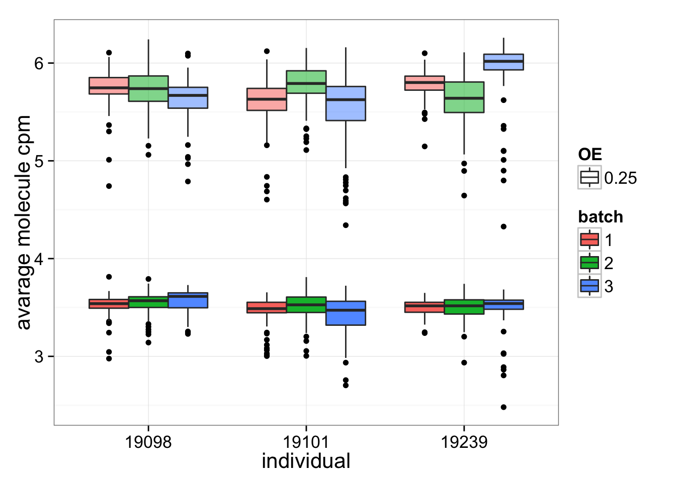
To answer the question if OE genes are more highly expressed, the average molecule CPM of OE genes or of all genes in each cells were plotted. If the OE genes are highly expressed, it is possible that this position effect is present in all genes but can only be observed with certain amount of expressing level.
## remove gene with 0 counts
expressed_single <- rowSums(molecules_single) > 0
molecules_single <- molecules_single[expressed_single, ]
dim(molecules_single)
[1] 17771 864## remove gene with molecule count larger than 1024 (15 if them)
overexpressed_genes <- rownames(molecules_single)[apply(molecules_single, 1,
function(x) any(x >= 1024))]
molecules_single <- molecules_single[!(rownames(molecules_single) %in% overexpressed_genes), ]
## collision probability and cpm molecule counts
molecules_single_collision <- -1024 * log(1 - molecules_single / 1024)
molecules_single_cpm <- cpm(molecules_single_collision, log = TRUE)
## select for OE genes
molecules_single_OE <- molecules_single_cpm[rownames(molecules_single_cpm) %in% as.character(OE_raw$genes),]
## boxplot
anno_single$OE_ave <- apply(molecules_single_OE, 2, mean)
anno_single$all_gene_ave <- apply(molecules_single_cpm, 2, mean)
ggplot(anno_single, aes(x = as.factor(individual))) + geom_boxplot(aes( y = OE_ave, fill = as.factor(batch), alpha = 0.25)) + geom_boxplot(aes( y = all_gene_ave, fill = as.factor(batch))) + labs (x = "individual", y = "avarage molecule cpm", alpha = "OE", fill = "batch")
Distribution of OE genes
cutoffs <- seq(1001, nrow(molecules_single_cpm), by = 1000)
cutoffs <- c(cutoffs, nrow(molecules_single_cpm))
top_genes_count <- lapply(1:length(cutoffs), function(cut) {
                        per_cutoff <- cutoffs[cut]
                        cell_across_order <- order(rowSums(molecules_single_cpm), decreasing = TRUE)
                        top_genes <- rownames(molecules_single_cpm)[cell_across_order < per_cutoff]
                        sum(OE_raw$genes %in% top_genes)
                        })
top_genes_count <- do.call(c, top_genes_count)

ggplot(data.frame(top_count = top_genes_count,
                  cutoffs = cutoffs),
       aes(x = as.factor(cutoffs), y = top_count)) + geom_point() +
       labs(x = "Top X genes", y = "Number of OEFinder OE genes")
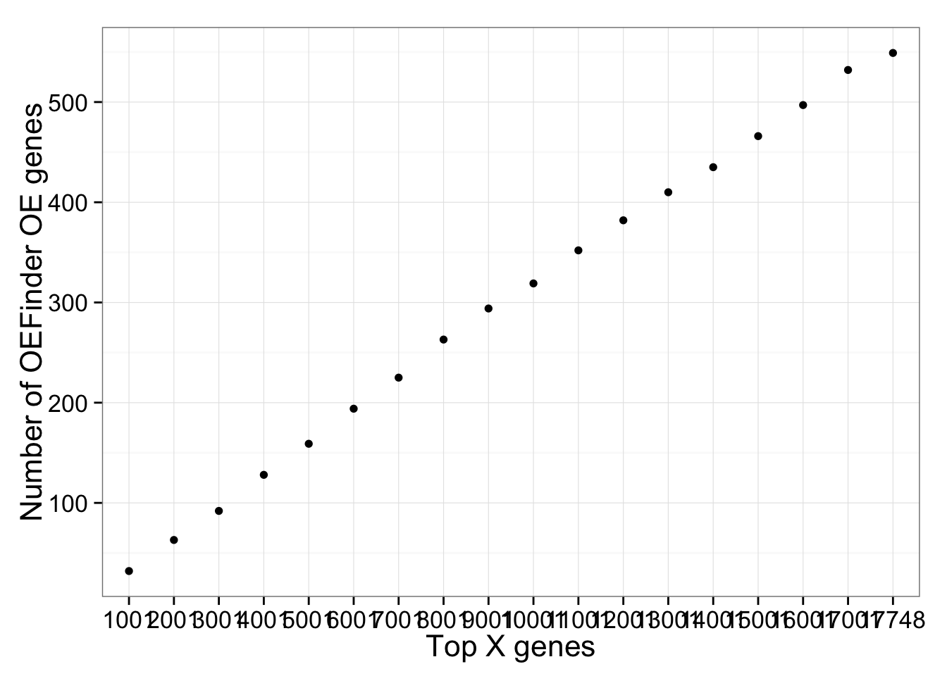
OE genes identified by OEFinder were not limited to the top 1000 genes. On the contrary, we found OE genes at all levels of gene expression (averaged acrosss cells).
Session information
sessionInfo()R version 3.2.1 (2015-06-18)
Platform: x86_64-apple-darwin13.4.0 (64-bit)
Running under: OS X 10.10.4 (Yosemite)
locale:
[1] en_US.UTF-8/en_US.UTF-8/en_US.UTF-8/C/en_US.UTF-8/en_US.UTF-8
=======
R version 3.2.0 (2015-04-16)
Platform: x86_64-unknown-linux-gnu (64-bit)
locale:
[1] LC_CTYPE=en_US.UTF-8 LC_NUMERIC=C
[3] LC_TIME=en_US.UTF-8 LC_COLLATE=en_US.UTF-8
[5] LC_MONETARY=en_US.UTF-8 LC_MESSAGES=en_US.UTF-8
[7] LC_PAPER=en_US.UTF-8 LC_NAME=C
[9] LC_ADDRESS=C LC_TELEPHONE=C
[11] LC_MEASUREMENT=en_US.UTF-8 LC_IDENTIFICATION=C
>>>>>>> 62bc5a2ab71c7d07af0b00504bd53484166fd98b
attached base packages:
[1] stats graphics grDevices utils datasets methods base
other attached packages:
<<<<<<< HEAD
[1] stringr_1.0.0 ggplot2_1.0.1 edgeR_3.10.2 limma_3.24.15 knitr_1.11
loaded via a namespace (and not attached):
[1] Rcpp_0.12.1 digest_0.6.8 MASS_7.3-44 grid_3.2.1
[5] plyr_1.8.3 gtable_0.1.2 formatR_1.2.1 magrittr_1.5
[9] scales_0.3.0 evaluate_0.8 stringi_0.5-5 reshape2_1.4.1
[13] rmarkdown_0.8 labeling_0.3 proto_0.3-10 tools_3.2.1
[17] munsell_0.4.2 yaml_2.1.13 colorspace_1.2-6 htmltools_0.2.6