Proportion of gene detected after filter

Setup

source("functions.R")
library("edgeR")

Loading required package: limma

library(ggplot2)
library("cowplot")

Attaching package: 'cowplot'

The following object is masked from 'package:ggplot2':

    ggsave

theme_set(theme_bw(base_size = 16))
theme_update(panel.grid.minor.x = element_blank(),
             panel.grid.minor.y = element_blank(),
             panel.grid.major.x = element_blank(),
             panel.grid.major.y = element_blank(),
             legend.key = element_blank(),
             plot.title = element_text(size = rel(1)))
require(matrixStats)

Loading required package: matrixStats
matrixStats v0.14.0 (2015-02-13) successfully loaded. See ?matrixStats for help.

Prepare single cell data

Input annotation

anno <- read.table("../data/annotation.txt", header = TRUE,
                   stringsAsFactors = FALSE)

anno_filter <- read.table("../data/annotation-filter.txt", header = TRUE,
                   stringsAsFactors = FALSE)

Input molecule counts

molecules <- read.table("../data/molecules.txt", header = TRUE,
           stringsAsFactors = FALSE)

molecules_filter <- read.table("../data/molecules-filter.txt", header = TRUE,
           stringsAsFactors = FALSE)

## qc cell
molecules_qc <- molecules[,colnames(molecules_filter)]
stopifnot(anno_filter$sample_id == colnames(molecules_qc))

Input read counts

reads <- read.table("../data/reads.txt", header = TRUE,
                    stringsAsFactors = FALSE)

reads_filter <- read.table("../data/reads-filter.txt", header = TRUE,
                    stringsAsFactors = FALSE)
## qc cell
reads_qc <- reads[,colnames(reads_filter)]
stopifnot(anno_filter$sample_id == colnames(reads_qc))

Molecule count data

First, look at the data set before removing lowly expressed genes (genes with low counts).

expressed_single <- rowSums(molecules_qc) > 0
expressed_single_reads <- rowSums(reads_qc) > 0

## stopifnot(expressed_single_reads == expressed_single)

molecules_single <- molecules_qc[which(expressed_single), ]
reads_single <- reads_qc[expressed_single_reads, ]

number_nonzero_cells <- colSums(molecules_single != 0)
number_genes <- dim(molecules_single)[1]
molecules_prop_genes_detected <- 
    data.frame(prop = number_nonzero_cells/number_genes,
               individual = anno_filter$individual,
               individual.batch = anno_filter$batch)

## create a color palette with one color per individual and different shades for repplicates
great_color <- c("#CC3300", "#FF9966", "#006633", "#009900", "#99FF99", "#3366FF", "#6699FF", "#66CCFF")

genes_detected_plot <- ggplot(molecules_prop_genes_detected,
                       aes(y = prop, x = as.factor(individual.batch), fill = as.factor(individual.batch))) + 
                       geom_boxplot(alpha = .01, width = .2, position = position_dodge(width = .9)) +
                       geom_violin(alpha = .5) + 
                       scale_fill_manual(values = great_color) +
                       labs(x = "Batch",
                       y = "Proportion of detected genes in single cell sample",
                       title = "Proportion of genes being detected across batch \n before filter") +
                       theme(axis.text.x = element_text(hjust=1, angle = 45))

Principal component analysis on cpm log2 transformed values. We avoid log of 0’s by add 1’s. In addition, our PCA analysis requires that every gene needs to be present in at least one of the cells.

## cpm 
molecules_single_cpm <- cpm(molecules_single)

## pca using log2 transformed data after adding 1
molecules_single_log2_pca <- run_pca( log2( molecules_single_cpm + 1))

pc1_plot <- qplot(y = molecules_single_log2_pca$PCs[,1],
      x = molecules_prop_genes_detected$prop,
      shape = as.factor(anno_filter$replicate),
      colour = as.factor(anno_filter$individual),
      xlab = "Proportion of genes detected",
      ylab = "PC1",
      title = "Proportion of genes detected") 

pc1_plot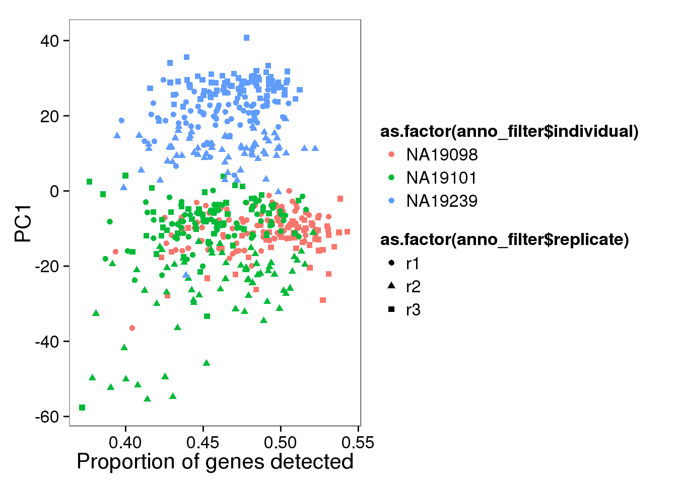

qplot(y = molecules_single_log2_pca$PCs[,2],
      x = molecules_prop_genes_detected$prop,
      shape = as.factor(anno_filter$replicate),
      colour = as.factor(anno_filter$individual),
      xlab = "Proportion of genes detected",
      ylab = "PC2")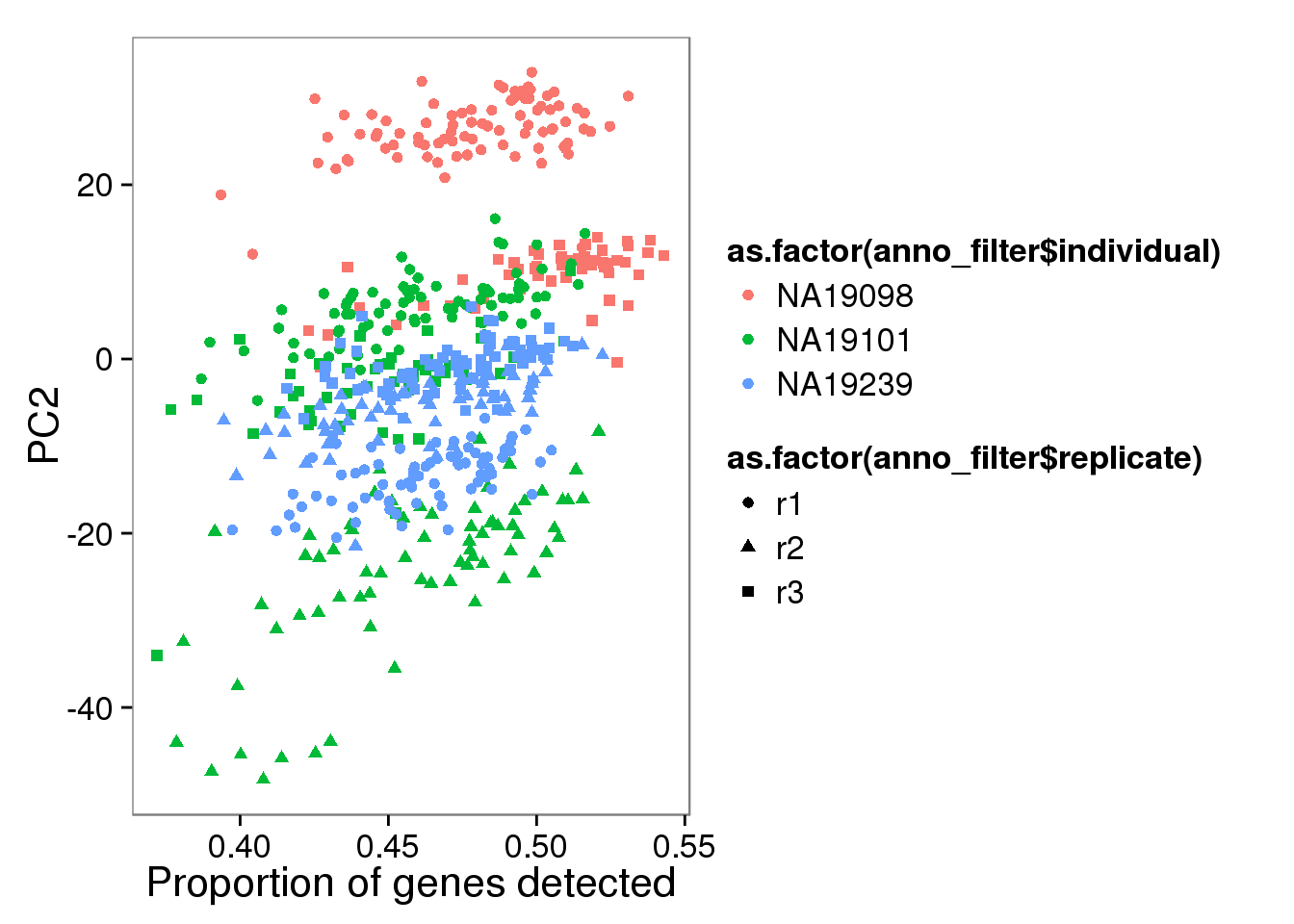 

Also look at the genes that were commonly detected in all cells to see if the the gene expression levels were involed as well.

# keep only genes detected in all cells
molecule_genes_all <- molecules_single[apply(molecules_single == 0, 1, sum) == 0 ,]
dim(molecule_genes_all)

[1] 1509  564

molecules_gene_all_pca <- run_pca( cpm(molecule_genes_all) )

pc1_plot_all <- qplot(y = molecules_gene_all_pca$PCs[,1],
      x = molecules_prop_genes_detected$prop,
      shape = as.factor(anno_filter$replicate),
      colour = as.factor(anno_filter$individual),
      xlab = "Proportion of genes detected",
      ylab = "PC1",
      title = "Proportion of genes detected") 

Molecule count data after filtering

Next, look at the data set after removing lowly expressed genes (genes with low counts).

number_nonzero_cells_filter <- colSums(molecules_filter != 0)
number_genes_filter <- dim(molecules_filter)[1]
molecules_prop_genes_detected_filter <- 
    data.frame(prop = number_nonzero_cells_filter/number_genes_filter,
               individual = anno_filter$individual,
               individual.batch = anno_filter$batch)

genes_detected_filter_plot <- ggplot(molecules_prop_genes_detected_filter,
                              aes(y = prop, x = as.factor(individual.batch), fill = as.factor(individual.batch))) + 
                              geom_boxplot(alpha = .01, width = .2, position = position_dodge(width = .9)) +
                              geom_violin(alpha = .5) + 
                              scale_fill_manual(values = great_color) +
                              labs(x = "Batch",
                                   y = "Proportion of detected genes in single cell sample",
                                   title = "Proportion of genes being detected across batch \n after filter") +
                              theme(axis.text.x = element_text(hjust=1, angle = 45))

### cpm 
molecules_filter_cpm <- cpm(molecules_filter)

## pca using log2 transformed data after adding 1
molecules_filter_log2_pca <- run_pca(log2 (molecules_filter_cpm + 1) )

pc1_filter_plot <- qplot(y = molecules_filter_log2_pca$PCs[,1],
      x = molecules_prop_genes_detected_filter$prop,
      shape = as.factor(anno_filter$replicate),
      colour = as.factor(anno_filter$individual),
      xlab = "Proportion of genes detected (filter)",
      ylab = "PC1",
      title = "Proportion of genes detected (filter)") 

pc1_filter_plot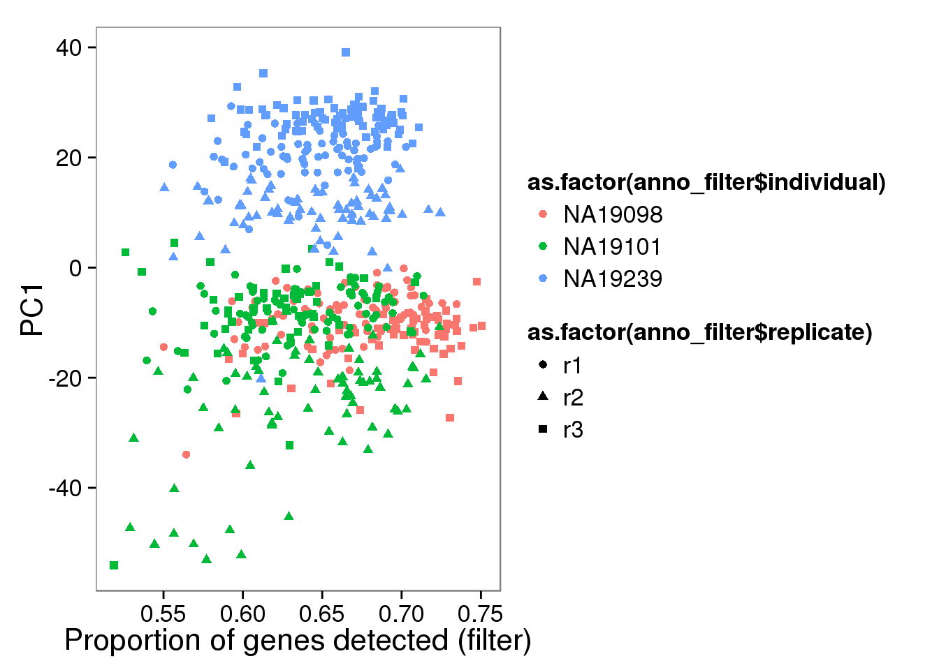

qplot(y = molecules_filter_log2_pca$PCs[,2],
      x = molecules_prop_genes_detected_filter$prop,
      shape = as.factor(anno_filter$replicate),
      colour = as.factor(anno_filter$individual),
      xlab = "Proportion of genes detected (filter)",
      ylab = "PC2")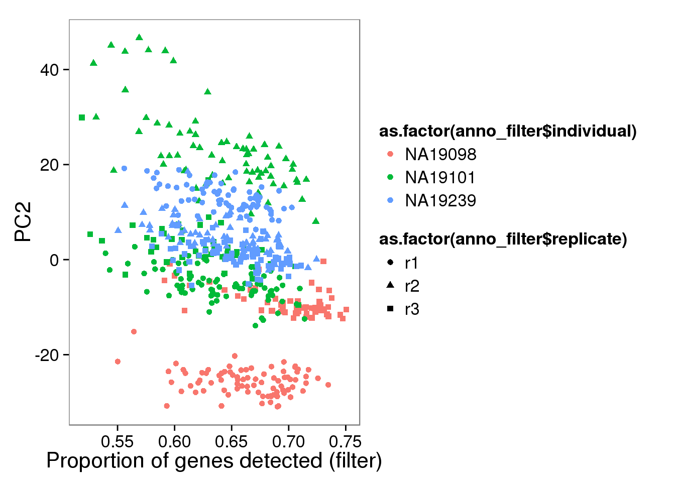 

# keep only genes detected in all cells
molecule_genes_all_filter <- molecules_filter[apply(molecules_filter == 0, 1, sum) == 0 ,]
dim(molecule_genes_all_filter)

[1] 1503  564

molecules_gene_all_filter_pca <- run_pca( cpm(molecule_genes_all_filter) )

pc1_plot_all_filter <- qplot(y = molecules_gene_all_filter_pca$PCs[,1],
      x = molecules_prop_genes_detected_filter$prop,
      shape = as.factor(anno_filter$replicate),
      colour = as.factor(anno_filter$individual),
      xlab = "Proportion of genes detected",
      ylab = "PC1",
      title = "Proportion of genes detected (filter)") 

Read counts data

number_nonzero_cells_reads <- colSums(reads_single != 0)
number_genes_reads <- dim(reads_single)[1]
reads_prop_genes_detected <- 
    data.frame(prop = number_nonzero_cells_reads/number_genes_reads,
               individual = anno_filter$individual,
               individual.batch = anno_filter$batch)

genes_detected_plot_reads <- ggplot(reads_prop_genes_detected,
                       aes(y = prop, x = as.factor(individual.batch), fill = as.factor(individual.batch))) + 
                       geom_boxplot(alpha = .01, width = .2, position = position_dodge(width = .9)) +
                       geom_violin(alpha = .5) + 
                       scale_fill_manual(values = great_color) +
                       labs(x = "Batch",
                       y = "Proportion of detected genes",
                       title = "Proportion of detected genes") +
                       theme(axis.text.x = element_text(hjust=1, angle = 45))

The effect of pseudocount in cpm

Code from Joyce :)

# this function computes PC1 of the inputted count matrix
# and also the correlation between the computed PC1
# and the proportion of genes detected.
pseudocount_pca <- function(pseudo_count, 
                            count_matrix,
                            gene_prop_detected_vector,
                            cor_method = "spearman", log_counts = FALSE) {
  # we use edgeR cpm function to compute normalized expression
  # a pseudo count is added to the count matrix if output is log expression
  # a pseudo is not added to the count matrix if output 
  if (log_counts == TRUE) {
      molecules_cpm <- log2(cpm(count_matrix, prior.count = pseudo_count) + 1) }
  if (log_counts == FALSE) {
      molecules_cpm <- cpm(count_matrix, prior.count = pseudo_count) }
  pc1 <- run_pca( (molecules_cpm))$PCs[,1]
  cor_coef <- cor(x = pc1, y = gene_prop_detected_vector, method = cor_method)
  return(list(pc1 = pc1, 
              cor_coef = cor_coef))
}

# specify pseudocount parameters
pseudo_count_vector <- c(10^(-5), 10^(-3), .1, .25, 1)

# use log-transformed normalized data
# compile results of the correlation between
# pc1 and proportion of genes detected
cor_pca_log <- lapply(1: length(pseudo_count_vector), function(ii) {
  obj <- pseudocount_pca(pseudo_count_vector[ii],
                          molecules_single,
                          molecules_prop_genes_detected$prop, log_counts = TRUE)
  return(obj)
})


# use normalized counts
# compile results of the correlation between
# pc1 and proportion of genes detected
cor_pca_count <- lapply(1: length(pseudo_count_vector), function(ii) {
  obj <- pseudocount_pca(pseudo_count_vector[ii],
                          molecules_single,
                          molecules_prop_genes_detected$prop, log_counts = FALSE)
  return(obj)
})


par(mfrow = c(1,2))
plot(x = pseudo_count_vector,
     y = sapply(cor_pca_log, function(xx) xx[[2]]))
plot(x = pseudo_count_vector,
     y = sapply(cor_pca_count, function(xx) xx[[2]]))

Summary plots

plot_grid(genes_detected_plot + theme(legend.position = "none"),
          genes_detected_filter_plot + theme(legend.position = "none"),
          pc1_plot + theme(legend.position = "none"),
          pc1_filter_plot + theme(legend.position = "none"),
          labels = letters[1:4],
          ncol = 2)

plot_grid(pc1_plot_all + theme(legend.position = "none"),
          pc1_plot_all_filter + theme(legend.position = "none"),
          labels = LETTERS[3:4])

Session information

sessionInfo()

R version 3.2.0 (2015-04-16)
Platform: x86_64-unknown-linux-gnu (64-bit)

locale:
 [1] LC_CTYPE=en_US.UTF-8       LC_NUMERIC=C              
 [3] LC_TIME=en_US.UTF-8        LC_COLLATE=en_US.UTF-8    
 [5] LC_MONETARY=en_US.UTF-8    LC_MESSAGES=en_US.UTF-8   
 [7] LC_PAPER=en_US.UTF-8       LC_NAME=C                 
 [9] LC_ADDRESS=C               LC_TELEPHONE=C            
[11] LC_MEASUREMENT=en_US.UTF-8 LC_IDENTIFICATION=C       

attached base packages:
[1] stats     graphics  grDevices utils     datasets  methods   base     

other attached packages:
[1] testit_0.4         matrixStats_0.14.0 cowplot_0.3.1     
[4] ggplot2_1.0.1      edgeR_3.10.2       limma_3.24.9      
[7] knitr_1.10.5      

loaded via a namespace (and not attached):
 [1] Rcpp_0.12.4      magrittr_1.5     MASS_7.3-40      munsell_0.4.3   
 [5] colorspace_1.2-6 stringr_1.0.0    httr_0.6.1       plyr_1.8.3      
 [9] tools_3.2.0      grid_3.2.0       gtable_0.1.2     htmltools_0.2.6 
[13] yaml_2.1.13      digest_0.6.8     reshape2_1.4.1   formatR_1.2     
[17] bitops_1.0-6     RCurl_1.95-4.6   evaluate_0.7     rmarkdown_0.6.1 
[21] labeling_0.3     stringi_1.0-1    scales_0.4.0     proto_0.3-10