Quality control at level of sequencing lane
John Blischak
2015-05-12
Last updated: 2015-06-11
Code version: 44338a0a5f347c0c7a565729f2a86161eb3229d3
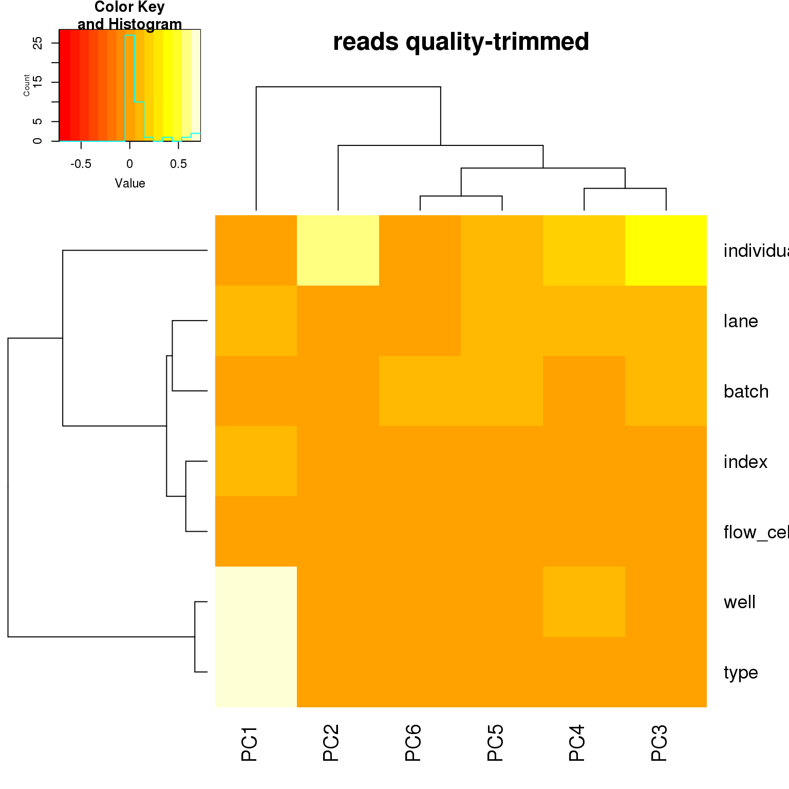
I performed PCA on the ERCC spike-ins to assess technical variability and a subset (~1000) of genes with a high coefficient of variation to assess the biological variability.
Conclusions:
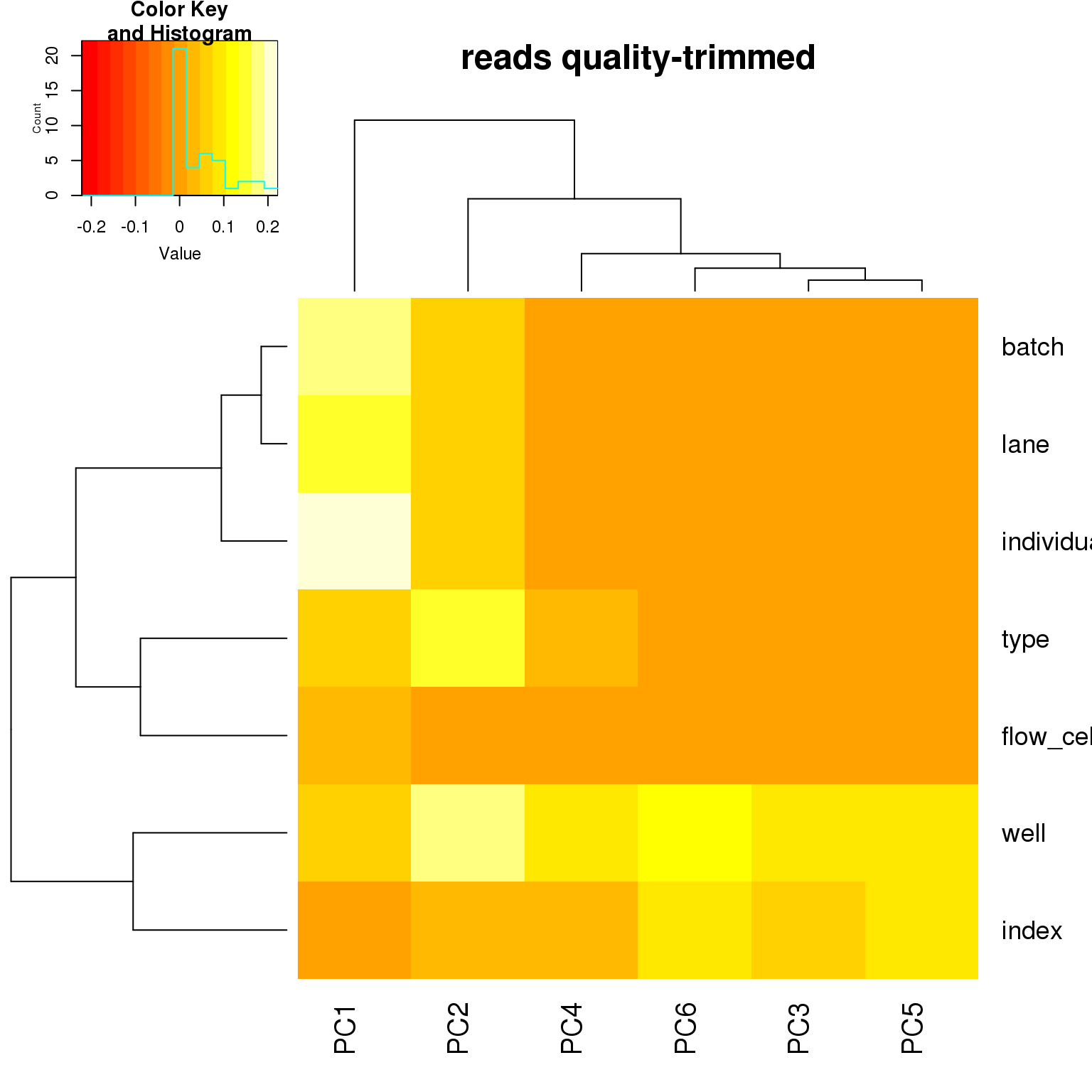
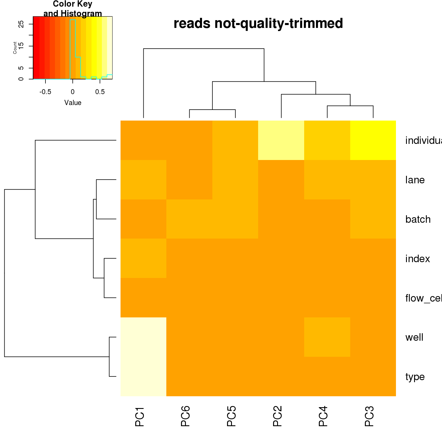
- No large difference in PCs whether or not reads are trimmed for quality at the 3’ end. Will use the quality trimmed data going forward.
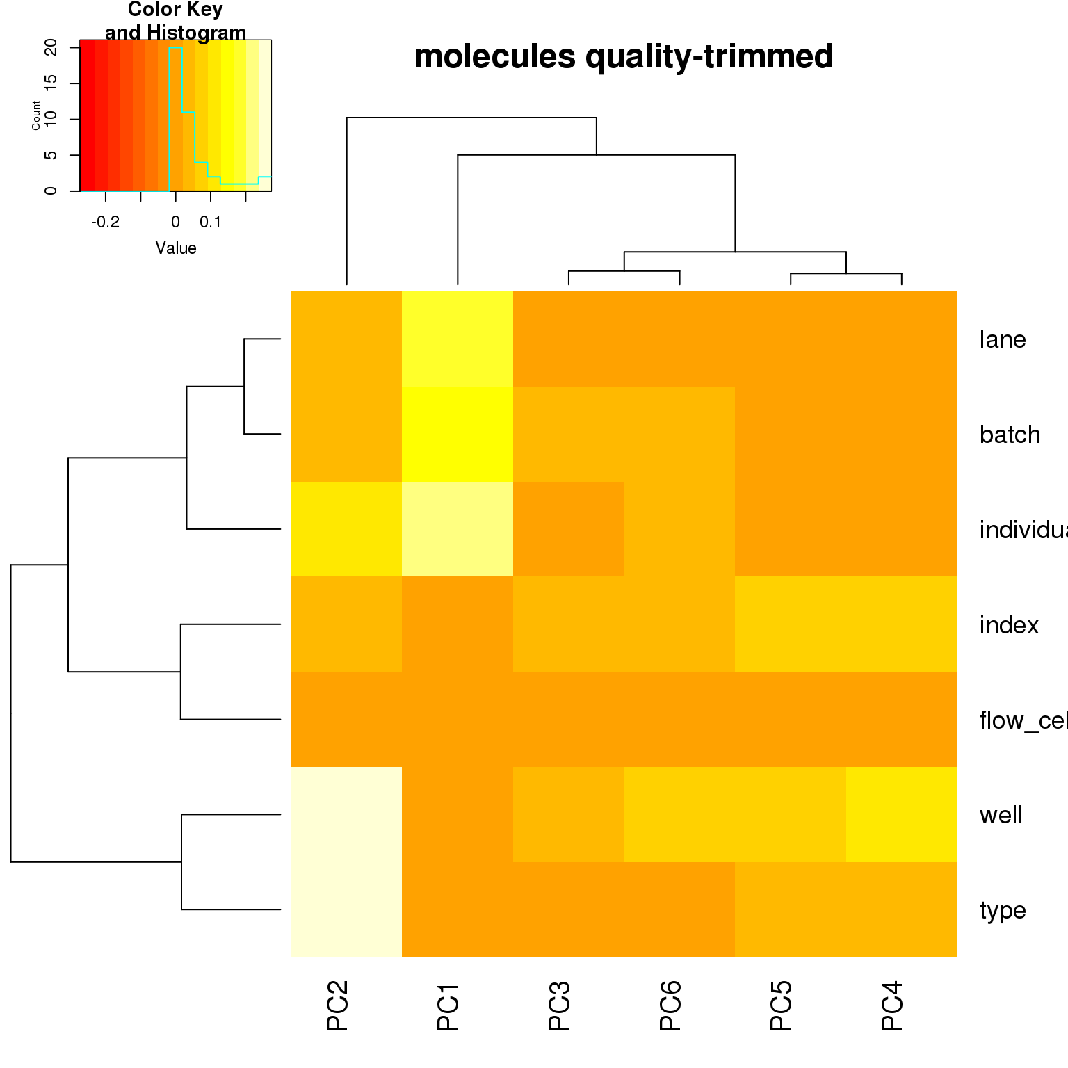
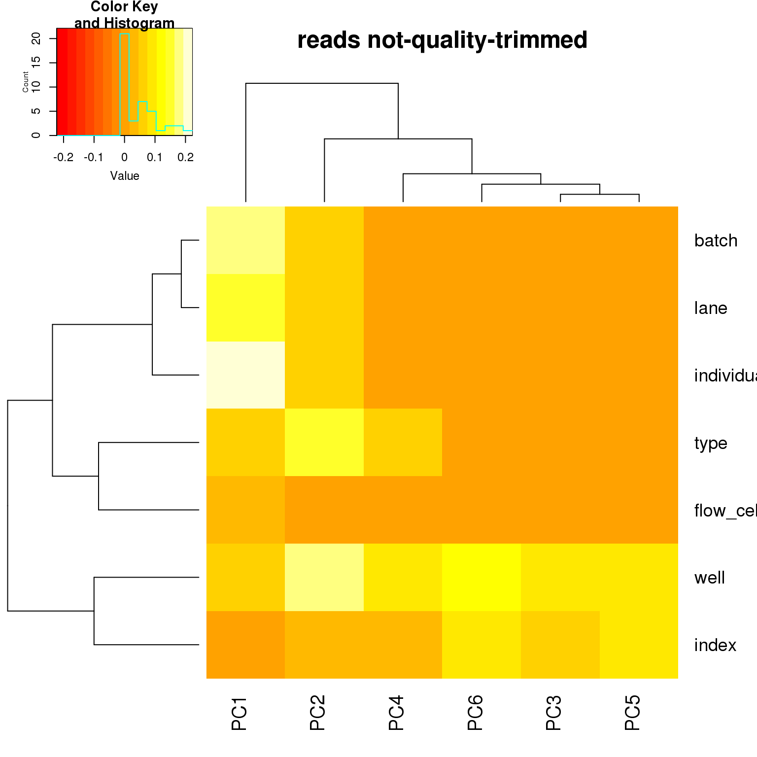
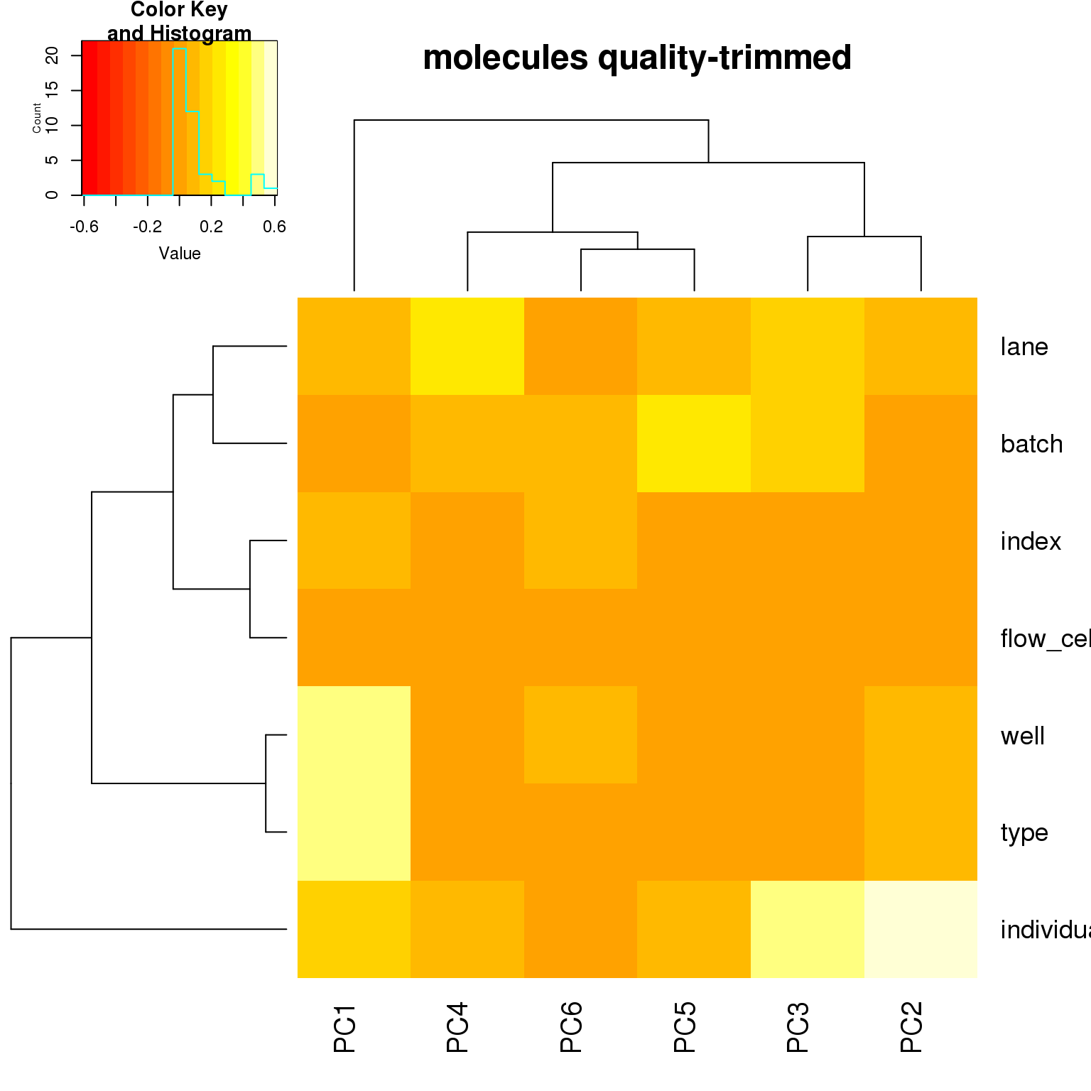
- For the ERCC data, the biggest effect on PC1 is individual, which appears to be driven by a subpopulation of the second batch of individual 19098. Need to investigate if these are dead cells.
- For the ERCC data, the biggest effect on the second PC is whether the sample is a bulk or single cell (represented by the factors
typeorwell) - For the variable genes, the biggest effect on PC1 is whether the sample is bulk or single cell, and the largest effect on PC2 is individual.
- Since there is no large obvious confounder to correct for, we will use sva to correct for technical effects.
Setup
The script gather-gene-counts.py compiles all the gene counts and extracts the relevant variables from the filename. The result is the file gene-counts.txt. Each row is a given fastq file (i.e. the sequences obtained for one from one lane of one flow cell), and each column is a variable (including all the genes).
library("data.table")
library("edgeR")
library("ggplot2")
library("gplots")
theme_set(theme_bw(base_size = 16))
counts <- fread("/mnt/gluster/data/internal_supp/singleCellSeq/gene-counts.txt")
Read 0.0% of 12402 rows
Read 80.6% of 12402 rows
Read 12402 rows and 20427 (of 20427) columns from 0.524 GB file in 00:00:30
Remove the combined samples. Only want to keep the per lane counts.
counts <- counts[!is.na(lane)]dim(counts)[1] 10656 20427head(counts[, 1:11, with = FALSE]) individual batch well index lane flow_cell sickle rmdup
1: 19098 1 A08 GAGCTCCA L003 C6WURACXX quality-trimmed reads
2: 19098 1 B07 TCAGTGTG L006 C723YACXX not-quality-trimmed reads
3: 19098 1 A06 GTCTGTAT L003 C6WURACXX quality-trimmed reads
4: 19098 1 B09 AAAGGTCC L002 C6WYKACXX not-quality-trimmed reads
5: 19098 1 C06 TCGGGTGA L002 C6WYKACXX not-quality-trimmed reads
6: 19098 1 F06 TCGCTAGT L003 C6WURACXX quality-trimmed reads
ENSG00000186092 ENSG00000237683 ENSG00000235249
1: 0 0 0
2: 0 0 0
3: 0 0 0
4: 0 0 0
5: 0 0 0
6: 0 0 0table(counts$lane, counts$flow_cell, counts$sickle, counts$rmdup), , = not-quality-trimmed, = molecules
C6WURACXX C6WYKACXX C723YACXX C72JMACXX
L001 96 18 96 96
L002 96 96 96 96
L003 96 96 96 96
L004 96 96 96 96
L005 96 96 18 96
L006 96 96 96 96
L007 96 96 96 0
L008 18 96 96 18
, , = quality-trimmed, = molecules
C6WURACXX C6WYKACXX C723YACXX C72JMACXX
L001 96 18 96 96
L002 96 96 96 96
L003 96 96 96 96
L004 96 96 96 96
L005 96 96 18 96
L006 96 96 96 96
L007 96 96 96 0
L008 18 96 96 18
, , = not-quality-trimmed, = reads
C6WURACXX C6WYKACXX C723YACXX C72JMACXX
L001 96 18 96 96
L002 96 96 96 96
L003 96 96 96 96
L004 96 96 96 96
L005 96 96 18 96
L006 96 96 96 96
L007 96 96 96 0
L008 18 96 96 18
, , = quality-trimmed, = reads
C6WURACXX C6WYKACXX C723YACXX C72JMACXX
L001 96 18 96 96
L002 96 96 96 96
L003 96 96 96 96
L004 96 96 96 96
L005 96 96 18 96
L006 96 96 96 96
L007 96 96 96 0
L008 18 96 96 18Functions
calc_pca <- function(dt, num_pcs = 1:6) {
  # Calculate pca.
  # dt - data.table
  # num_pcs: Number of PCs to return
  require("edgeR")
  stopifnot(class(dt)[1] == "data.table")
  dt <- dt[, colSums(dt) > 0, with = FALSE]
  dt <- t(dt)
  cpm_mat <- cpm(dt, log = TRUE)
  pca <- prcomp(t(cpm_mat), scale. = TRUE)
  # return(as.list(pca$x))
  return(pca$x[, num_pcs])
}
calc_pca_by_subset <- function(counts, anno, num_pcs = 1:6) {
# Calculate pca for 4 subsets:
# quality-trimmed reads
# quality-trimmed molecules
# not-quality-trimmed reads
# not-quality-trimmed molecules
# counts: data.table of counts with rows = samples and columns = genes
# anno: annotation file with rows = samples and columns = categorical variables
# num_pcs: Number of PCs to return
# Returns data.frame with PCs plus annotation
stopifnot(class(counts)[1] == "data.table",
class(anno)[1] == "data.table")
pca <- data.frame()
for (rmdup_status in c("molecules", "reads")) {
for (sickle_status in c("not-quality-trimmed", "quality-trimmed")) {
dat <- counts[anno$rmdup == rmdup_status & anno$sickle == sickle_status, ]
# print(dat[, .N])
result <- calc_pca(dat, num_pcs = num_pcs)
result_df <- data.frame(anno[rmdup == rmdup_status & sickle == sickle_status, ], result,
stringsAsFactors = FALSE)
pca <- rbind(pca, result_df)
}
}
return(pca)
}correlate_pcs <- function(pca) {
# Plot heatmaps of adjusted r-squared values from simple linear regression between PCs
# and categorical variables.
# pca: data.frame of PCs plus annotation
factors <- colnames(pca)[c(1:6, 9)]
pcs <- colnames(pca)[10:ncol(pca)]
for (rmdup_status in c("molecules", "reads")) {
for (sickle_status in c("not-quality-trimmed", "quality-trimmed")) {
pca_corr <- matrix(NA, nrow = length(factors), ncol = length(pcs),
dimnames = list(factors, pcs))
for (fac in factors) {
for (pc in pcs) {
result_lm <- lm(pca[pca$rmdup == rmdup_status &
pca$sickle == sickle_status, pc] ~
as.factor(pca[pca$rmdup == rmdup_status &
pca$sickle == sickle_status, fac]))
result_r2 <- summary(result_lm)$adj.r.squared
# result_df <- data.frame(fac, pc, result_r2, stringsAsFactors = FALSE)
pca_corr[fac, pc] <- result_r2
}
}
heatmap.2(pca_corr, trace = "none", main = paste(rmdup_status, sickle_status))
}
}
}PCA on ERCC spike-ins
Using only the ERCC control genes for PCA. Should isolate purely technical effects.
counts_ercc <- counts[, grep("ERCC", colnames(counts)), with = FALSE]
anno <- counts[, 1:8, with = FALSE]
anno$type <- ifelse(anno$well == "bulk", "bulk", "single")
pca_ercc <- calc_pca_by_subset(counts_ercc, anno)ggplot(pca_ercc, aes(x = PC1, y = PC2, col = as.factor(type))) +
geom_point() +
facet_grid(sickle ~ rmdup)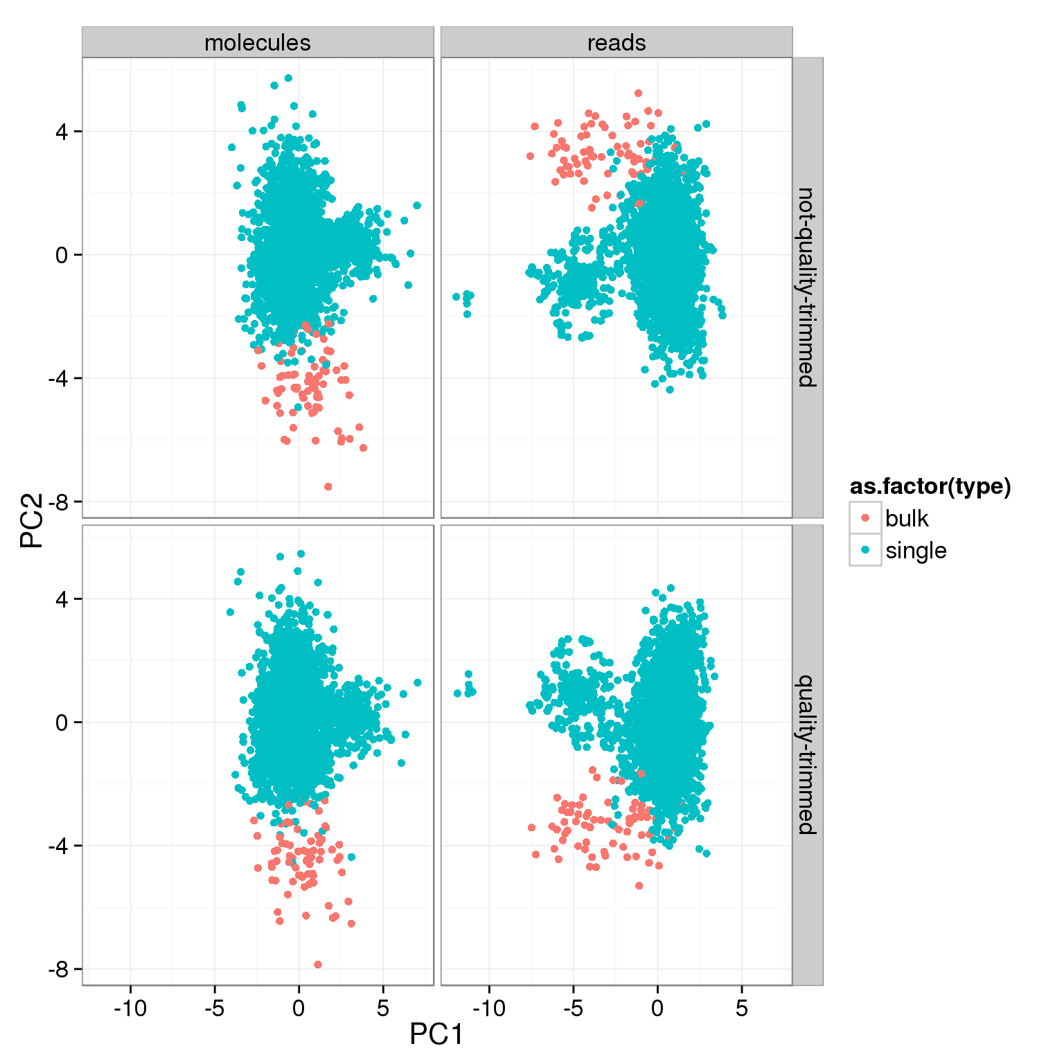
ggplot(pca_ercc, aes(x = PC1, y = PC2, col = as.factor(individual), shape = as.factor(batch))) +
  geom_point(size = 3, alpha = 0.5) +
  facet_grid(sickle ~ rmdup)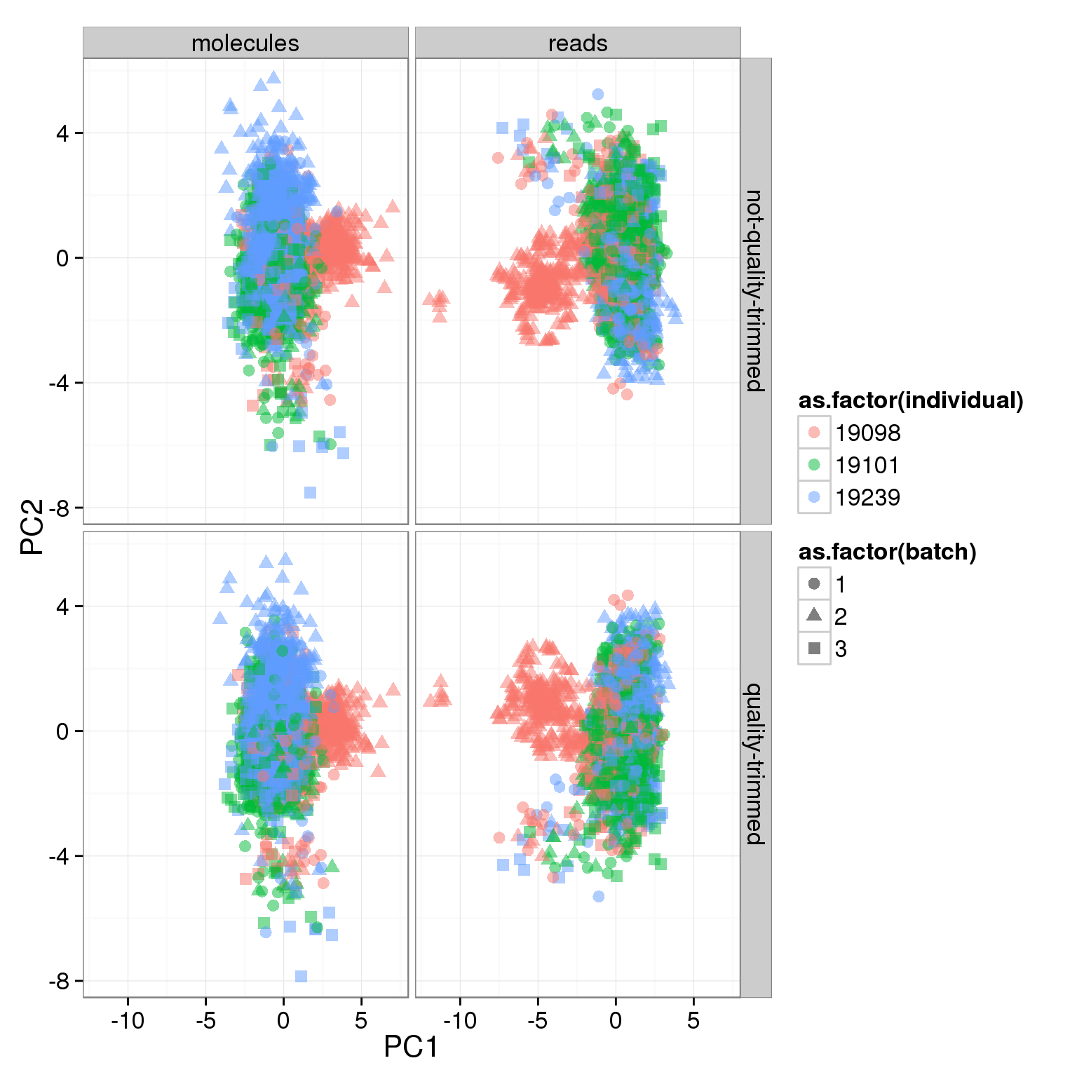
ggplot(pca_ercc, aes(x = PC1, y = PC2, col = as.factor(batch))) +
  geom_point(size = 3, alpha = 0.5) +
  facet_grid(sickle ~ rmdup)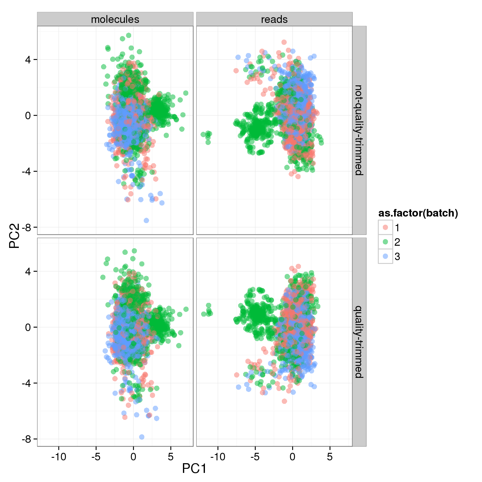
correlate_pcs(pca_ercc)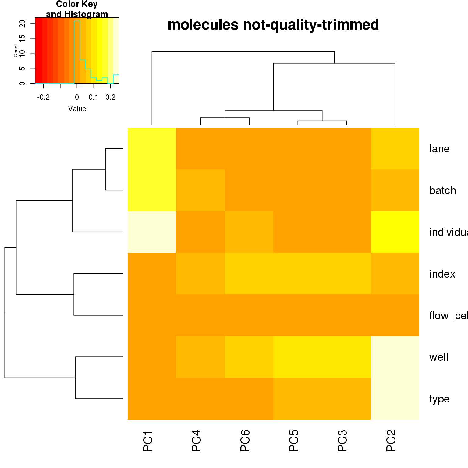
PCA on highly variable genes
It is too computationally intensive to perform PCA on thousands of genes. Instead limiting to genes with a high coefficient of variation for the non-quality-trimmed reads.
Find most variable genes
cov <- counts[, lapply(.SD, function(x) sd(x) / (mean(x) + 1)),
              by = .(rmdup, sickle),
              .SDcols = grep("ENSG", colnames(counts))]
cov_reads_not_qual <- cov[rmdup == "reads" & sickle == "not-quality-trimmed",
                          grep("ENSG", colnames(cov)), with = FALSE]
cov_vec <- as.numeric(cov_reads_not_qual)
names(cov_vec) <- colnames(cov_reads_not_qual)
var_genes <- names(cov_vec)[cov_vec > 3]
PCA using variable genes
counts_cov <- counts[, var_genes, with = FALSE]pca_cov <- calc_pca_by_subset(counts_cov, anno)ggplot(pca_cov, aes(x = PC1, y = PC2, col = as.factor(type))) +
geom_point() +
facet_grid(sickle ~ rmdup)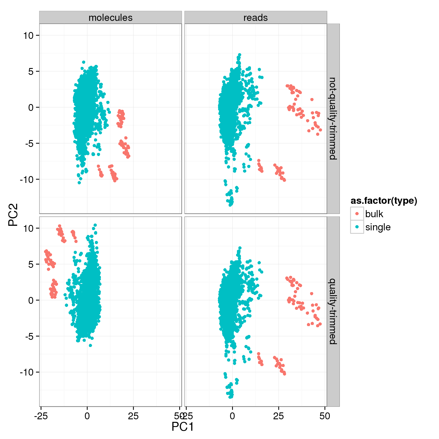
ggplot(pca_cov, aes(x = PC1, y = PC2, col = as.factor(individual))) +
  geom_point() +
  facet_grid(sickle ~ rmdup)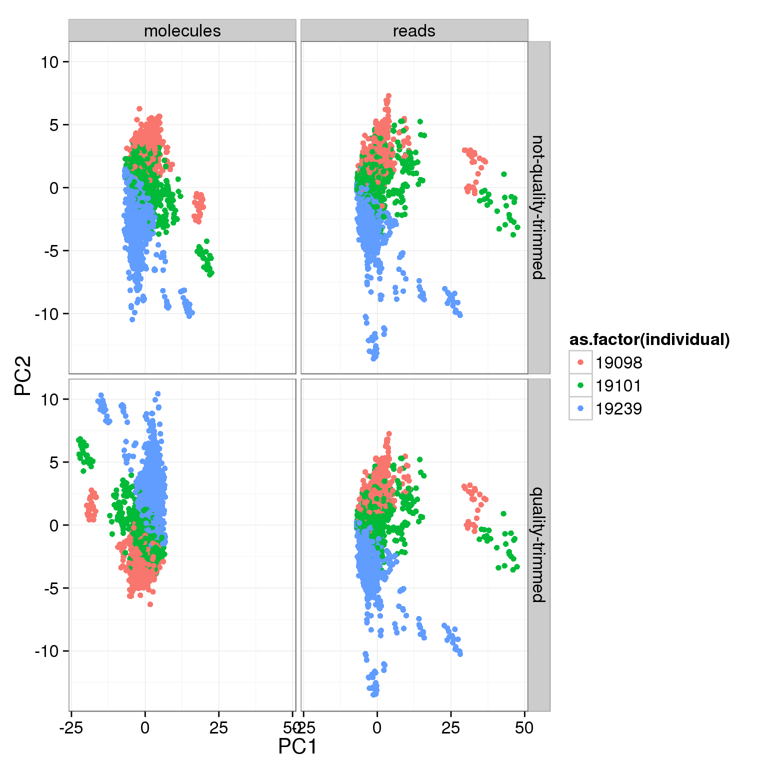
correlate_pcs(pca_cov)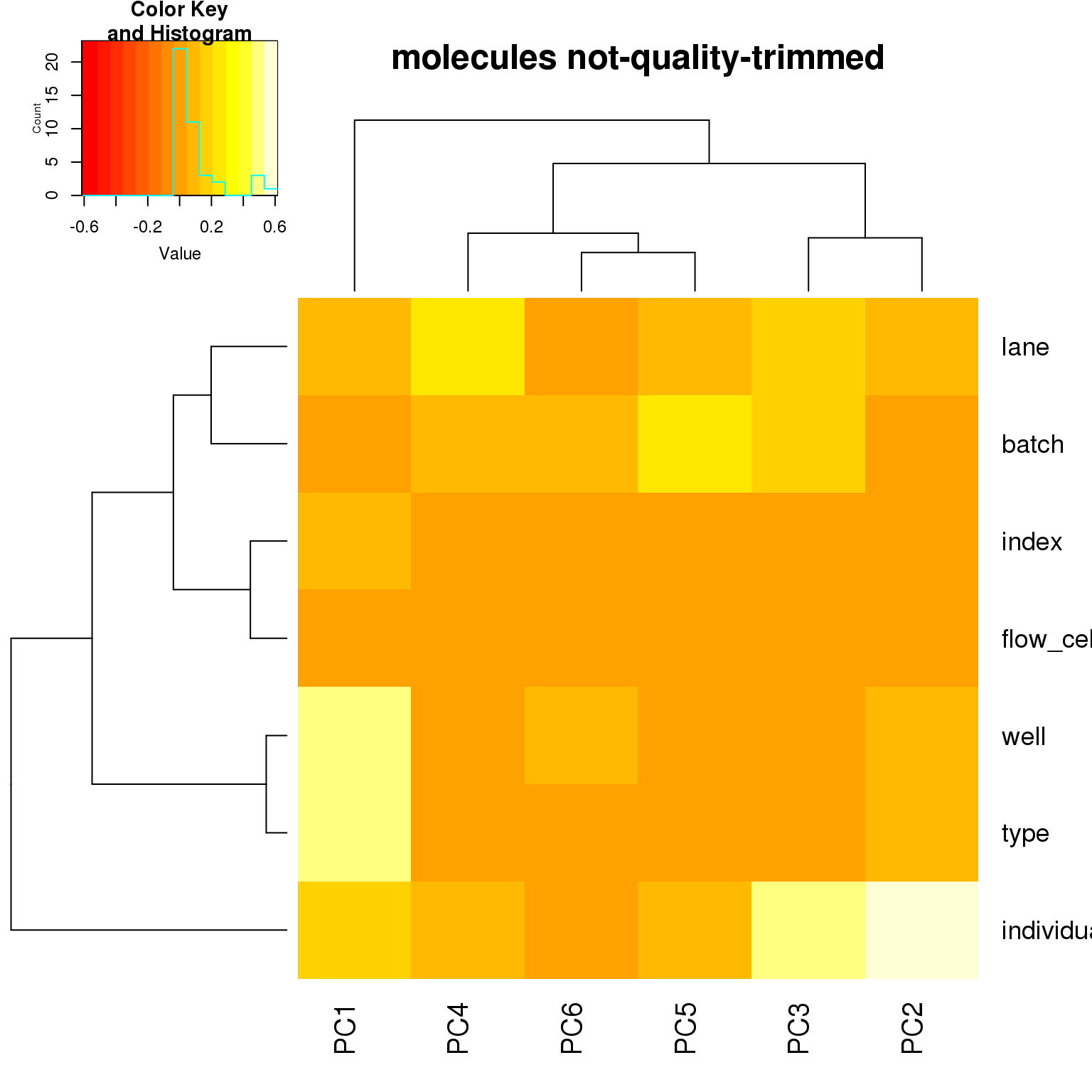
Session information
sessionInfo()R version 3.2.0 (2015-04-16)
Platform: x86_64-unknown-linux-gnu (64-bit)
locale:
[1] LC_CTYPE=en_US.UTF-8 LC_NUMERIC=C
[3] LC_TIME=en_US.UTF-8 LC_COLLATE=en_US.UTF-8
[5] LC_MONETARY=en_US.UTF-8 LC_MESSAGES=en_US.UTF-8
[7] LC_PAPER=en_US.UTF-8 LC_NAME=C
[9] LC_ADDRESS=C LC_TELEPHONE=C
[11] LC_MEASUREMENT=en_US.UTF-8 LC_IDENTIFICATION=C
attached base packages:
[1] stats graphics grDevices utils datasets methods base
other attached packages:
[1] gplots_2.17.0 ggplot2_1.0.1 edgeR_3.10.2 limma_3.24.9
[5] data.table_1.9.4 knitr_1.10.5
loaded via a namespace (and not attached):
[1] Rcpp_0.11.6 magrittr_1.5 MASS_7.3-40
[4] munsell_0.4.2 colorspace_1.2-6 stringr_1.0.0
[7] plyr_1.8.2 caTools_1.17.1 tools_3.2.0
[10] grid_3.2.0 gtable_0.1.2 KernSmooth_2.23-14
[13] gtools_3.5.0 htmltools_0.2.6 yaml_2.1.13
[16] digest_0.6.8 reshape2_1.4.1 formatR_1.2
[19] bitops_1.0-6 evaluate_0.7 rmarkdown_0.6.1
[22] labeling_0.3 gdata_2.16.1 stringi_0.4-1
[25] scales_0.2.4 chron_2.3-45 proto_0.3-10