QC of single cell libraries
PoYuan Tung
2015-10-23
Last updated: 2016-11-08
Code version: bd286a36f14d3b332285cdc7e62258b1f616bb14
Input
library("dplyr")
library("edgeR")
library("ggplot2")
library("cowplot")
theme_set(theme_bw(base_size = 16))
theme_update(panel.grid.minor.x = element_blank(),
             panel.grid.minor.y = element_blank(),
             panel.grid.major.x = element_blank(),
             panel.grid.major.y = element_blank(),
             legend.key = element_blank(),
             plot.title = element_text(size = rel(1)))
source("functions.R")
Summary counts from featureCounts. Created with gather-summary-counts.py. These data were collected from the summary files of the full combined samples.
summary_per_sample <- read.table("../data/summary-counts.txt", header = TRUE,
                             stringsAsFactors = FALSE)
stopifnot(summary_per_sample$well != "bulk",
          sum(summary_per_sample$rmdup == "reads") == 864,
          sum(summary_per_sample$rmdup == "molecules") == 864)
Remove featureCounts classifications with zero counts.
stopifnot(colSums(summary_per_sample[, c(7, 10:15)]) == 0)
summary_per_sample <- summary_per_sample[, c(-7, -10:-15)]
head(summary_per_sample)
individual replicate well rmdup Assigned Unassigned_Ambiguity
1 NA19098 r1 A01 molecules 63322 1419
2 NA19098 r1 A01 reads 1932782 40278
3 NA19098 r1 A02 molecules 63976 1454
4 NA19098 r1 A02 reads 2039613 44664
5 NA19098 r1 A03 molecules 43630 976
6 NA19098 r1 A03 reads 1006487 18865
Unassigned_NoFeatures Unassigned_Unmapped
1 54297 0
2 885075 1093943
3 49595 0
4 737166 1140902
5 33597 0
6 419226 742614Input annotation.
anno <- read.table("../data/annotation.txt", header = TRUE,
                   stringsAsFactors = FALSE)
stopifnot(anno$well != "bulk", nrow(anno) == 864,
          rep(anno$individual, each = 2) == summary_per_sample$individual,
          rep(anno$replicate, each = 2) == summary_per_sample$replicate,
          rep(anno$well, each = 2) == summary_per_sample$well)
head(anno)
individual replicate well batch sample_id
1 NA19098 r1 A01 NA19098.r1 NA19098.r1.A01
2 NA19098 r1 A02 NA19098.r1 NA19098.r1.A02
3 NA19098 r1 A03 NA19098.r1 NA19098.r1.A03
4 NA19098 r1 A04 NA19098.r1 NA19098.r1.A04
5 NA19098 r1 A05 NA19098.r1 NA19098.r1.A05
6 NA19098 r1 A06 NA19098.r1 NA19098.r1.A06Input read counts.
reads <- read.table("../data/reads.txt", header = TRUE,
                    stringsAsFactors = FALSE)
stopifnot(ncol(reads) == nrow(anno),
          colnames(reads) == anno$sample_id)
Input molecule counts.
molecules <- read.table("../data/molecules.txt", header = TRUE,
                    stringsAsFactors = FALSE)
stopifnot(ncol(molecules) == nrow(anno),
          colnames(reads) == anno$sample_id)
Input single cell observational quality control data.
qc <- read.table("../data/qc-ipsc.txt", header = TRUE,
                 stringsAsFactors = FALSE)
stopifnot(qc$individual == anno$individual,
          qc$replicate == anno$replicate,
          qc$well == anno$well)
head(qc)
individual replicate well cell_number concentration tra1.60
1 NA19098 r1 A01 1 1.734785 1
2 NA19098 r1 A02 1 1.723038 1
3 NA19098 r1 A03 1 1.512786 1
4 NA19098 r1 A04 1 1.347492 1
5 NA19098 r1 A05 1 2.313047 1
6 NA19098 r1 A06 1 2.056803 1Total ERCC and removal of NA19098.r2
Show the evidence that removing NA19098 batch 2 is the first thing to do.
summary_per_sample_reads <- summary_per_sample[summary_per_sample$rmdup == "reads",]

summary_per_sample_reads$sample_id <- anno$sample_id
summary_per_sample_reads$batch <- anno$batch
stopifnot(colnames(reads) == summary_per_sample_reads$sample_id )

summary_per_sample_reads$ERCC_reads <- apply(reads[grep("ERCC", rownames(reads)), ],2,sum)
summary_per_sample_reads$ERCC_molecules <- apply(molecules[grep("ERCC", rownames(molecules)), ],2,sum)
## create a color palette with one color per individual and different shades for repplicates
great_color <- c("#CC3300", "#FF9966", "#FFCC99", "#006633", "#009900", "#99FF99", "#3366FF", "#6699FF", "#66CCFF")
great_color_8 <- c("#CC3300", "#FF9966", "#006633", "#009900", "#99FF99", "#3366FF", "#6699FF", "#66CCFF")
ercc_reads_plot <- ggplot(summary_per_sample_reads,
aes(x = factor(batch), y = ERCC_reads,
fill = factor(batch)), height = 600, width = 2000) +
geom_violin(alpha = .5) +
geom_boxplot(alpha = .01, width = .2, position = position_dodge(width = .9)) +
scale_fill_manual(values = great_color) +
labs(x = "", y = "Total ERCC read-counts per cell",
title = "Excess amount of ERCC in NA19098.r2") +
theme(axis.text.x = element_text(hjust=1, angle = 45))
ercc_molecule_plot <- ggplot(summary_per_sample_reads,
aes(x = factor(batch), y = ERCC_molecules,
fill = factor(batch)), height = 600, width = 2000) +
geom_violin(alpha = .5) +
geom_boxplot(alpha = .01, width = .2, position = position_dodge(width = .9)) +
scale_fill_manual(values = great_color) +
labs(x = "", y = "Total ERCC molecule-counts per cell",
title = "Excess amount of ERCC in NA19098.r2") +
theme(axis.text.x = element_text(hjust=1, angle = 45))
plot_grid(ercc_reads_plot + theme(legend.position=c(.8,.7)),
ercc_molecule_plot + theme(legend.position = "none"),
labels = LETTERS[1:2])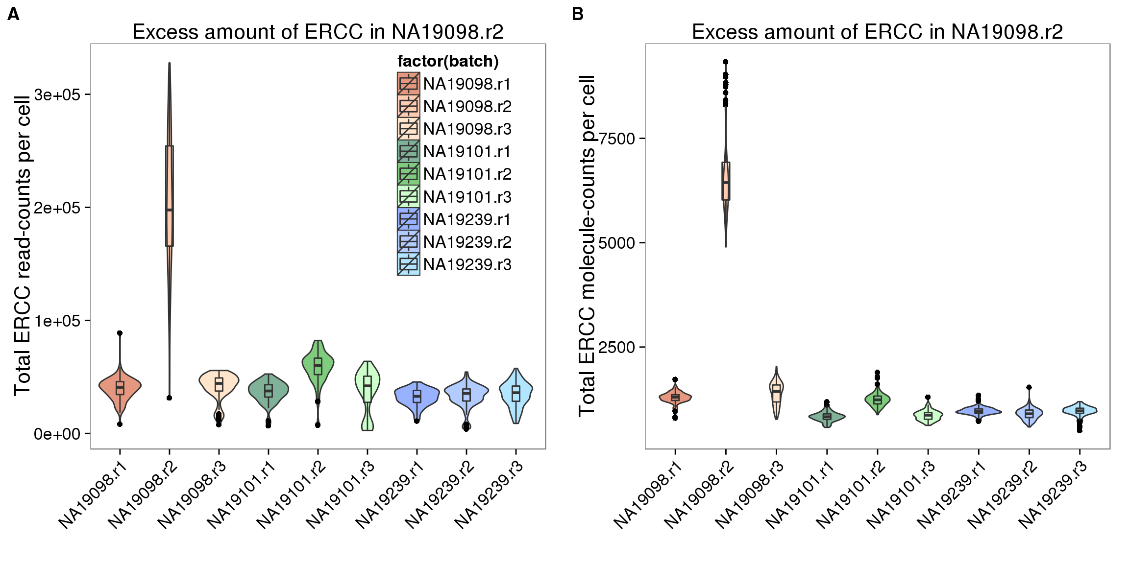
Remove NA19098r2 for all the following analysis
remove_19098r2 <- anno$batch != "NA19098.r2"
anno_rm <- anno[remove_19098r2,]
summary_per_sample_reads_rm <- summary_per_sample_reads[remove_19098r2,]
reads_rm <- reads[, remove_19098r2]
molecules_rm <- molecules[, remove_19098r2]

stopifnot(summary_per_sample_reads_rm$sample_id == colnames(reads_rm))
Total mapped reads reads
## add cell number per well by merging qc file
summary_per_sample_reads_qc <- merge(summary_per_sample_reads_rm,qc,by=c("individual","replicate","well"))

## calculate total mapped reads per sample
summary_per_sample_reads_qc$total_mapped <- apply(summary_per_sample_reads_qc[,5:7],1,sum)

## cut off
cut_off_reads <- quantile(summary_per_sample_reads_qc[summary_per_sample_reads_qc$cell_number == 0,"total_mapped"], 0.95)

cut_off_reads
95%
1556255 summary_per_sample_reads_qc$cut_off_reads <- summary_per_sample_reads_qc$total_mapped > cut_off_reads
## numbers of cells
sum(summary_per_sample_reads_qc[summary_per_sample_reads_qc$cell_number == 1, "total_mapped"] > cut_off_reads)[1] 603sum(summary_per_sample_reads_qc[summary_per_sample_reads_qc$cell_number == 1, "total_mapped"] <= cut_off_reads)[1] 96## density plots
plot_reads <- ggplot(summary_per_sample_reads_qc[summary_per_sample_reads_qc$cell_number == 0 |
summary_per_sample_reads_qc$cell_number == 1 , ],
aes(x = total_mapped, fill = as.factor(cell_number))) +
geom_density(alpha = 0.5) +
geom_vline(xintercept = cut_off_reads, colour="grey", linetype = "longdash") +
labs(x = "Total mapped reads per sample", title = "Cutoff based on the number of total mapped reads", fill = "Cell number")Unmapped ratios
## calculate unmapped ratios
summary_per_sample_reads_qc$unmapped_ratios <- summary_per_sample_reads_qc[,8]/apply(summary_per_sample_reads_qc[,5:8],1,sum)

## cut off
cut_off_unmapped <- quantile(summary_per_sample_reads_qc[summary_per_sample_reads_qc$cell_number == 0,"unmapped_ratios"], 0.05)

cut_off_unmapped
5%
0.3640165 summary_per_sample_reads_qc$cut_off_unmapped <- summary_per_sample_reads_qc$unmapped_ratios < cut_off_unmapped
## numbers of cells
sum(summary_per_sample_reads_qc[summary_per_sample_reads_qc$cell_number == 1, "unmapped_ratios"] >= cut_off_unmapped)[1] 101sum(summary_per_sample_reads_qc[summary_per_sample_reads_qc$cell_number == 1, "unmapped_ratios"] < cut_off_unmapped)[1] 598## density plots
plot_unmapped <- ggplot(summary_per_sample_reads_qc[summary_per_sample_reads_qc$cell_number == 0 |
summary_per_sample_reads_qc$cell_number == 1 , ],
aes(x = unmapped_ratios *100, fill = as.factor(cell_number))) +
geom_density(alpha = 0.5) +
geom_vline(xintercept = cut_off_unmapped *100, colour="grey", linetype = "longdash") +
labs(x = "Unmapped reads / Total reads per sample", title = "Cutoff based on the percentage unmapped reads")ERCC percentage
## calculate ercc reads percentage
summary_per_sample_reads_qc$ercc_percentage <- apply(reads_rm[grep("ERCC", rownames(reads_rm)), ],2,sum)/apply(summary_per_sample_reads_qc[,5:7],1,sum)

## cut off
cut_off_ercc <- quantile(summary_per_sample_reads_qc[summary_per_sample_reads_qc$cell_number == 0,"ercc_percentage"], 0.05)

cut_off_ercc
5%
0.0323008 summary_per_sample_reads_qc$cut_off_ercc <- summary_per_sample_reads_qc$ercc_percentage < cut_off_ercc
## numbers of cells
sum(summary_per_sample_reads_qc[summary_per_sample_reads_qc$cell_number == 1, "ercc_percentage"] >= cut_off_ercc)[1] 90sum(summary_per_sample_reads_qc[summary_per_sample_reads_qc$cell_number == 1, "ercc_percentage"] < cut_off_ercc)[1] 609## density plots
plot_ercc <- ggplot(summary_per_sample_reads_qc[summary_per_sample_reads_qc$cell_number == 0 |
summary_per_sample_reads_qc$cell_number == 1 , ],
aes(x = ercc_percentage *100, fill = as.factor(cell_number))) +
geom_density(alpha = 0.5) +
geom_vline(xintercept = cut_off_ercc *100, colour="grey", linetype = "longdash") +
labs(x = "ERCC reads / Total mapped reads per sample", title = "Cutoff based on the percentage of ERCC reads")Number of genes detected
## endogenous genes
reads_rm_gene <- reads_rm[grep("ENSG", rownames(reads_rm)), ]

## number of genes detected
summary_per_sample_reads_qc$gene_number <- colSums(reads_rm_gene >= 1)

## cut off
cut_off_genes <- quantile(summary_per_sample_reads_qc[summary_per_sample_reads_qc$cell_number == 0,"gene_number"], 0.95)

cut_off_genes
95%
6788.9 summary_per_sample_reads_qc$cut_off_genes <- summary_per_sample_reads_qc$gene_number > cut_off_genes
## numbers of cells
sum(summary_per_sample_reads_qc[summary_per_sample_reads_qc$cell_number == 1, "gene_number"] > cut_off_genes)[1] 629sum(summary_per_sample_reads_qc[summary_per_sample_reads_qc$cell_number == 1, "gene_number"] <= cut_off_genes)[1] 70## density plots
plot_gene <- ggplot(summary_per_sample_reads_qc[summary_per_sample_reads_qc$cell_number == 0 |
summary_per_sample_reads_qc$cell_number == 1 , ],
aes(x = gene_number, fill = as.factor(cell_number))) +
geom_density(alpha = 0.5) +
geom_vline(xintercept = cut_off_genes, colour="grey", linetype = "longdash") +
labs(x = "Gene numbers per sample", title = "Cutoff based on the number of detected genes")plot_grid(plot_reads + theme(legend.position=c(.7,.7)),
plot_unmapped + theme(legend.position = "none"),
plot_ercc + theme(legend.position = "none"),
plot_gene + theme(legend.position = "none"),
labels = LETTERS[3:6])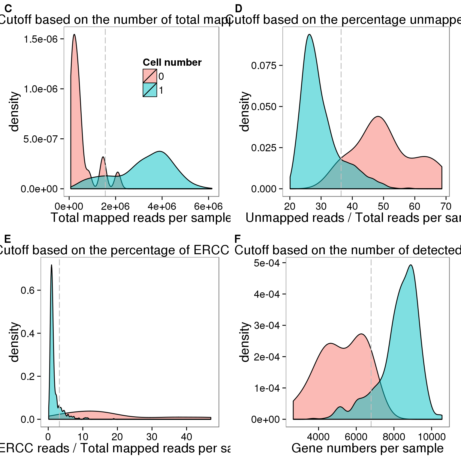
Total molecule counts
## calculate total gene molecule counts
summary_per_sample_reads_qc$total_gene_molecule <- colSums(molecules_rm[grep("ENSG", rownames(molecules_rm)),])

## look for outiers
ggplot(summary_per_sample_reads_qc, aes(x = concentration, y = total_gene_molecule / 10^3,
  color = as.factor(cell_number))) +
  geom_text(aes(label = cell_number)) +
  labs(x = "Concentration", y = "Gene molecules (thousands)") +
  scale_color_brewer(palette = "Dark2") +
  theme(legend.position = "none")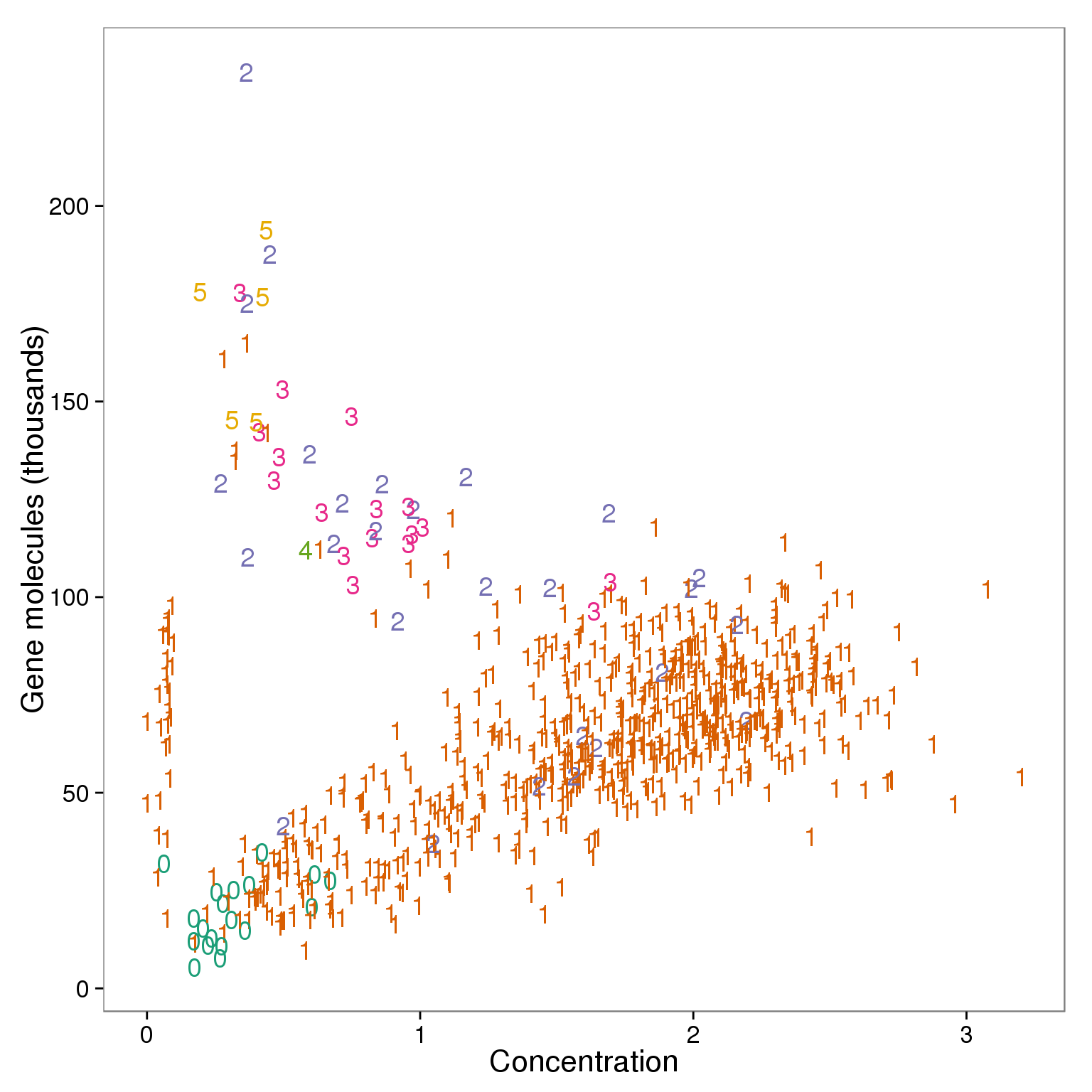
outliers <- summary_per_sample_reads_qc %>% filter(cell_number == 1, concentration < 1.25, concentration > .15,
                                   total_gene_molecule > 100000)

outliers %>% dplyr::select(sample_id)
sample_id
1 NA19098.r3.B04
2 NA19098.r3.B11
3 NA19101.r1.B10
4 NA19101.r2.D07
5 NA19101.r3.C07
6 NA19101.r3.D08
7 NA19101.r3.F05
8 NA19101.r3.F10
9 NA19239.r2.A12
10 NA19239.r2.B07Linear Discriminant Analysis
library(MASS)
Attaching package: 'MASS'

The following object is masked from 'package:dplyr':

    select
## create 3 groups according to cell number
group_3 <- rep("multiple cells",dim(summary_per_sample_reads_qc)[1])
group_3[grep("0", summary_per_sample_reads_qc$cell_number)] <- "no cells"
group_3[grep("1", summary_per_sample_reads_qc$cell_number)] <- "one cell"
## create data frame
data_lda <- data.frame(anno_rm,
cell_number = summary_per_sample_reads_qc$cell_number,
concentration = summary_per_sample_reads_qc$concentration,
total_gene_molecule = summary_per_sample_reads_qc$total_gene_molecule,
group = group_3)
## remove 19098.r1
data_con <- data_lda %>% filter(batch != "NA19098.r1")
plot_before <- ggplot(data_con, aes(x = concentration, y = total_gene_molecule / 10^3,
color = as.factor(group))) +
geom_text(aes(label = cell_number)) +
labs(x = "Sample concentration",
y = "Total gene molecule-count per sample (thousands)",
title = "Before linear discriminant analysis (LDA) \n A few samples with one cell (purple) \n clustered with samples with multiple cells (green)") +
scale_color_brewer(palette = "Dark2") +
theme(legend.position = "none")
## perform lda
data_con_lda <- lda(group ~ concentration + total_gene_molecule,
data = data_con)
data_con_lda_p <- predict(data_con_lda,
newdata = data_con[,c("concentration", "total_gene_molecule")])$class
## determine how well the model fix
table(data_con_lda_p, data_con[, "group"])
data_con_lda_p   multiple cells no cells one cell
  multiple cells             34        0       10
  no cells                    0        1        0
  one cell                   15       16      596
data_con$data_con_lda_p <- data_con_lda_p
plot_after <- ggplot(data_con, aes(x = concentration, y = total_gene_molecule / 10^3,
color = as.factor(data_con_lda_p))) +
geom_text(aes(label = cell_number)) +
labs(x = "Sample concentration",
y = "Total gene molecule-count per sample (thousands)",
title = "After linear discriminant analysis (LDA) \n Removal of samples classified as \n samples with multiple cells (green)") +
scale_color_brewer(palette = "Dark2") +
theme(legend.position = "none")
## identify the outlier
outliers_lda <- data_con %>% filter(cell_number == 1, data_con_lda_p == "multiple cells")
outliers_lda$sample_id [1] "NA19098.r3.B04" "NA19098.r3.B11" "NA19101.r1.B10" "NA19101.r2.D07"
[5] "NA19101.r3.C07" "NA19101.r3.D08" "NA19101.r3.F05" "NA19101.r3.F10"
[9] "NA19239.r2.A12" "NA19239.r2.B07"## The lds method identifies outliers
plot_grid(plot_before + theme(legend.position=c(.8,.85)),
plot_after + theme(legend.position = "none"),
labels = LETTERS[1:2])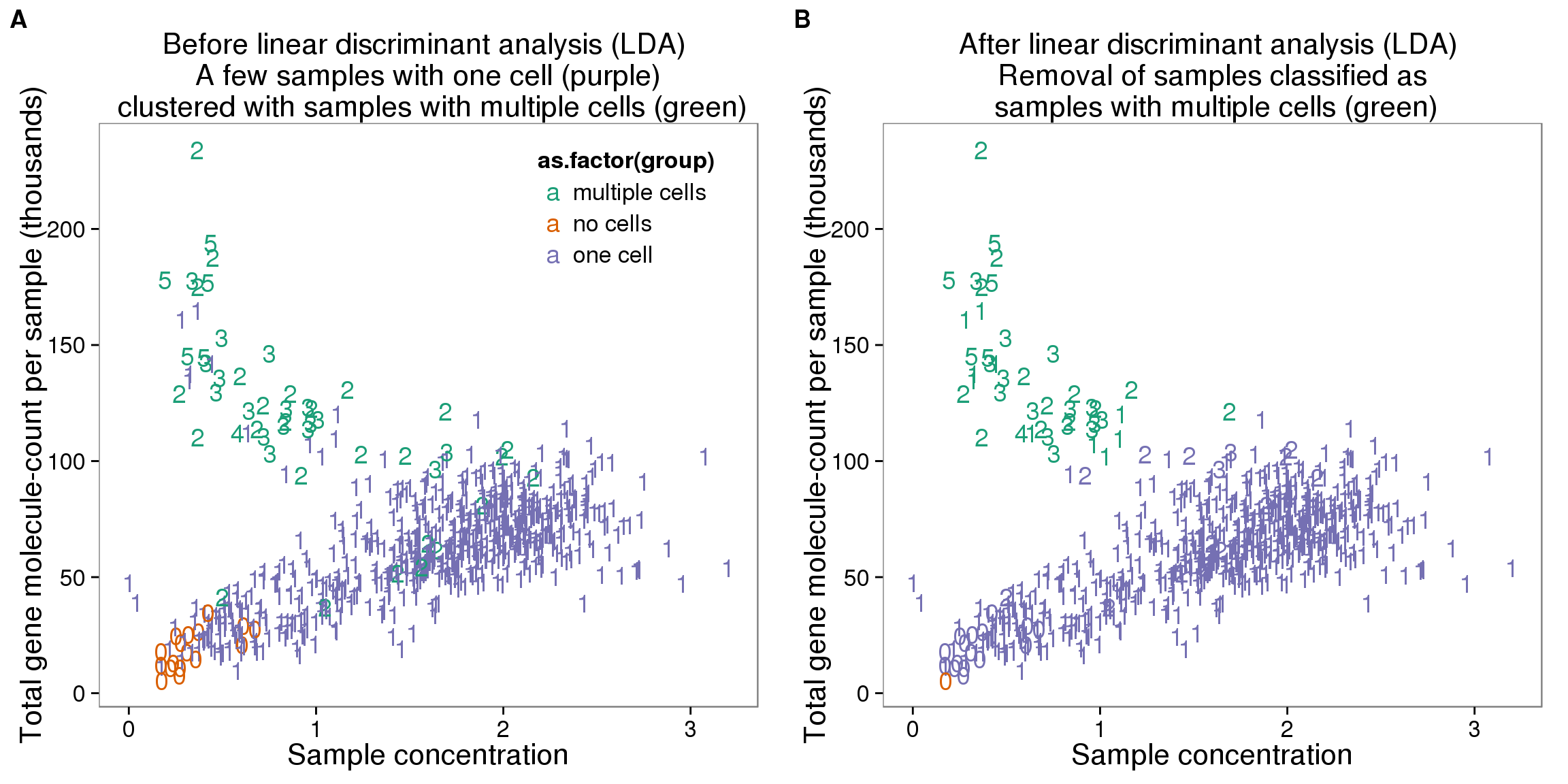
## create filter
summary_per_sample_reads_qc$molecule_outlier <- summary_per_sample_reads_qc$sample_id %in% outliers_lda$sample_id
Reads to molecule conversion
## calculate convertion
summary_per_sample_reads_qc$ERCC_conversion <- summary_per_sample_reads_qc$ERCC_molecules / summary_per_sample_reads_qc$ERCC_reads

summary_per_sample_reads_qc$conversion <- summary_per_sample_reads_qc$total_gene_molecule /  colSums(reads_rm[grep("ENSG", rownames(reads_rm)),])

ggplot(summary_per_sample_reads_qc, aes(x = ERCC_conversion, y = conversion,
  color = as.factor(cell_number))) +
  geom_text(aes(label = cell_number)) +
  labs(x = "Convertion of ERCC", y = "Conversion of genes") +
  scale_color_brewer(palette = "Dark2") +
  theme(legend.position = "none")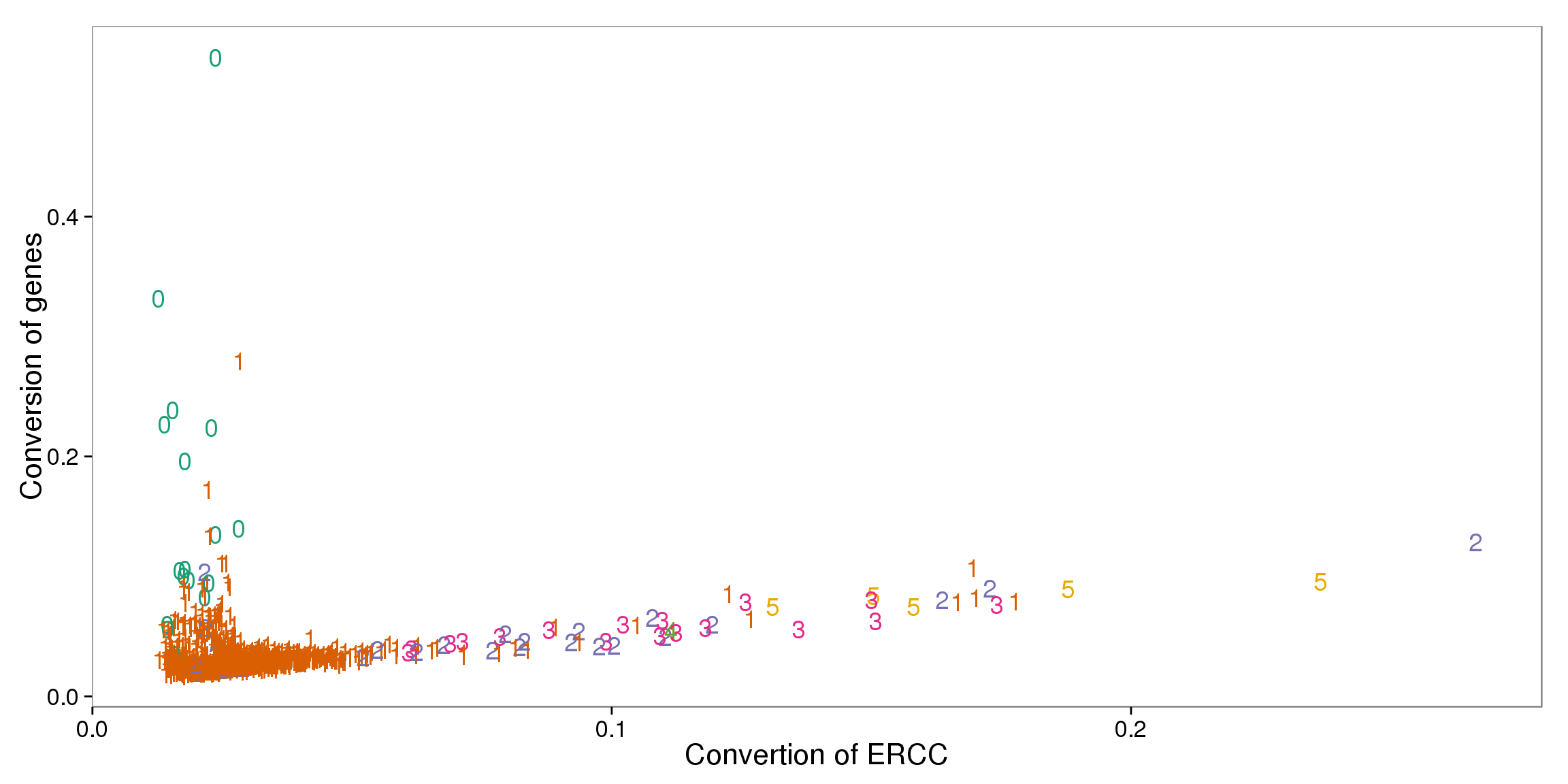
out_ercc_con <- summary_per_sample_reads_qc %>% filter(cell_number == "1", ERCC_conversion > .094)

## try lda
data_lda$conversion <- summary_per_sample_reads_qc$conversion
data_lda$ERCC_conversion <- summary_per_sample_reads_qc$ERCC_conversion

data_ercc_lda <- lda(group ~ ERCC_conversion + conversion,
                    data = data_lda)
data_ercc_lda_p <- predict(data_ercc_lda,
                          newdata = data_lda[,c("ERCC_conversion", "conversion")])$class
table(data_con_lda_p, data_con[, "group"])
data_con_lda_p   multiple cells no cells one cell
  multiple cells             34        0       10
  no cells                    0        1        0
  one cell                   15       16      596
data_lda$data_ercc_lda_p <- data_ercc_lda_p
## identify the outlier
outliers_ercc <- data_lda %>% filter(cell_number == 1, data_ercc_lda_p == "multiple cells")
outliers_ercc$sample_id [1] "NA19098.r1.F01" "NA19098.r3.B04" "NA19098.r3.B11" "NA19101.r2.D07"
[5] "NA19101.r3.C07" "NA19101.r3.D08" "NA19101.r3.F05" "NA19101.r3.F10"
[9] "NA19239.r2.A12" "NA19239.r2.B07" "NA19239.r3.G02"## cutoff
out_ercc_con <- summary_per_sample_reads_qc %>% filter(cell_number == "1", ERCC_conversion > .08)
## create filter
summary_per_sample_reads_qc$conversion_outlier <- summary_per_sample_reads_qc$sample_id %in% outliers_ercc$sample_id
plot_ercc_before <- ggplot(data_lda, aes(x = ERCC_conversion, y = conversion,
color = as.factor(group))) +
geom_text(aes(label = cell_number)) +
labs(x = "Read-to-molecule conversion of ERCC",
y = "Read-to-molecule conversion of genes",
title = "Before linear discriminant analysis (LDA) \n A few samples with one cell (purple) \n clustered with samples with multiple cells (green)") +
scale_color_brewer(palette = "Dark2") +
theme(legend.position = "none")
plot_ercc_after <- ggplot(data_lda, aes(x = ERCC_conversion, y = conversion,
color = as.factor(data_ercc_lda_p))) +
geom_text(aes(label = cell_number)) +
labs(x = "Read-to-molecule conversion of ERCC",
y = "Read-to-molecule conversion of genes",
title = "After linear discriminant analysis (LDA) \n Removal of samples classified as \n samples with multiple cells (green)") +
scale_color_brewer(palette = "Dark2") +
theme(legend.position = "none")
plot_grid(plot_ercc_before,
plot_ercc_after,
labels = LETTERS[3:4])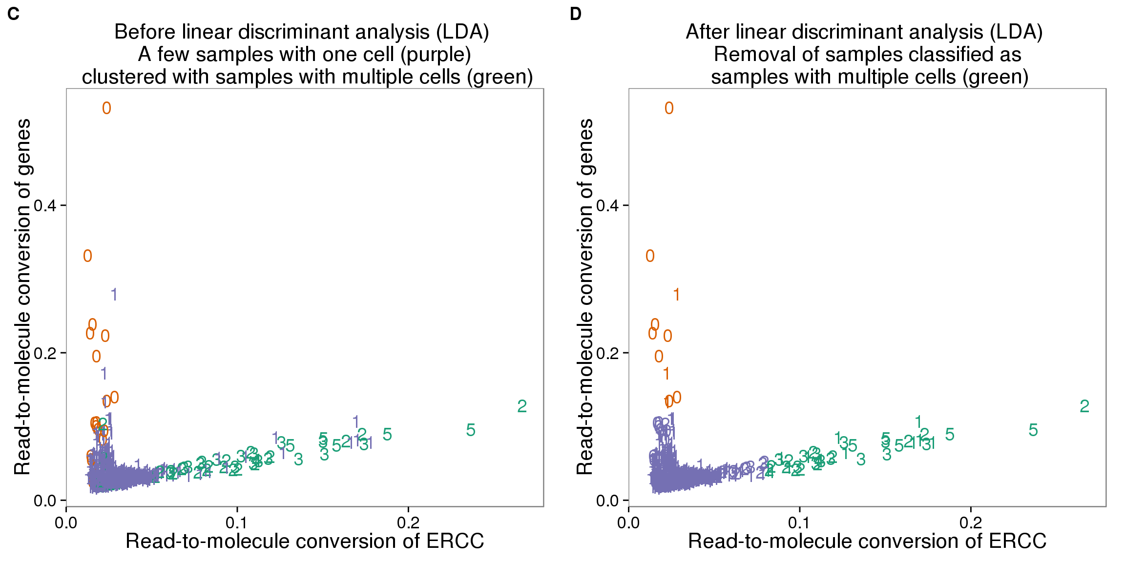
Mitochondrial genes
## create a list of mitochondrial genes (13 protein-coding genes)
## MT-ATP6, MT-CYB, MT-ND1, MT-ND4, MT-ND4L, MT-ND5, MT-ND6, MT-CO2, MT-CO1, MT-ND2, MT-ATP8, MT-CO3, MT-ND3
mtgene <- c("ENSG00000198899", "ENSG00000198727", "ENSG00000198888", "ENSG00000198886", "ENSG00000212907", "ENSG00000198786", "ENSG00000198695", "ENSG00000198712", "ENSG00000198804", "ENSG00000198763","ENSG00000228253", "ENSG00000198938", "ENSG00000198840")

## reads of mt genes in single cells
mt_reads <- reads_rm_gene[mtgene,]
dim(mt_reads)
[1] 13 768stopifnot(colnames(reads_rm) == rownames(summary_per_sample_reads_qc$sample_id))
## mt ratio of single cell
summary_per_sample_reads_qc$mt_reads <- apply(mt_reads, 2, sum)
summary_per_sample_reads_qc$mt_reads_ratio <- summary_per_sample_reads_qc$mt_reads /summary_per_sample_reads_qc$total_mapped
## vs. number of genes detected
ggplot(summary_per_sample_reads_qc,
aes(x = gene_number, y = mt_reads_ratio,
color = as.factor(cell_number))) +
geom_text(aes(label = cell_number)) +
labs(x = "Number of genes", y = "Mitochondrial ratio") +
scale_color_brewer(palette = "Dark2") +
theme(legend.position = "none")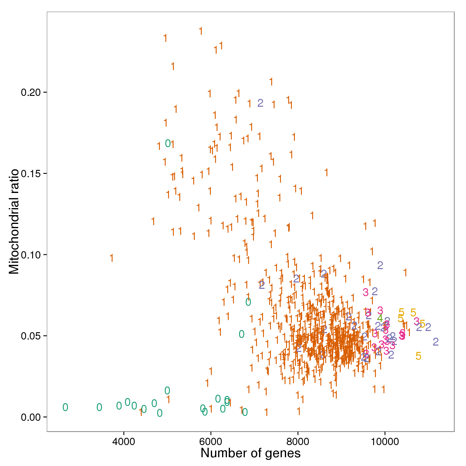
Filter
Final list
## all filter
summary_per_sample_reads_qc$filter_all <- summary_per_sample_reads_qc$cell_number == 1 &
                                                 summary_per_sample_reads_qc$cut_off_reads &
                                                 summary_per_sample_reads_qc$cut_off_unmapped &
                                                 summary_per_sample_reads_qc$cut_off_ercc &
                                                 summary_per_sample_reads_qc$cut_off_genes &
                                                 summary_per_sample_reads_qc$molecule_outlier == "FALSE" &
                                                 summary_per_sample_reads_qc$conversion_outlier == "FALSE"

table(summary_per_sample_reads_qc[summary_per_sample_reads_qc$filter_all,
                           c("individual", "replicate")])
replicate
individual r1 r2 r3
NA19098 85 0 57
NA19101 80 70 51
NA19239 74 68 79stopifnot(nrow(summary_per_sample_reads_qc) == nrow(anno_rm))
quality_single_cells <- anno_rm %>%
filter(summary_per_sample_reads_qc$filter_all) %>%
dplyr :: select(sample_id)
write.table(quality_single_cells,
file = "../data/quality-single-cells.txt", quote = FALSE,
sep = "\t", row.names = FALSE, col.names = FALSE)Mito ratios
ggplot(summary_per_sample_reads_qc,
       aes(x = gene_number, y = mt_reads_ratio,
       color = as.factor(filter_all))) +
       geom_text(aes(label = cell_number)) +
       labs(x = "Number of genes", y = "Mitochondrial ratio") +
       theme(legend.position = "none")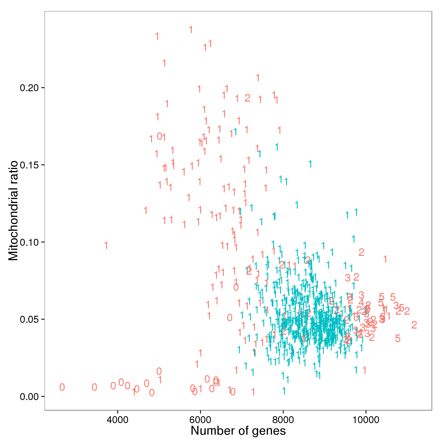
ggplot(summary_per_sample_reads_qc[summary_per_sample_reads_qc$cell_number == 1,],
       aes(x = factor(filter_all), y = mt_reads_ratio,
           fill = factor(filter_all)), height = 600, width = 2000) +
geom_violin(alpha = .5) +
geom_boxplot(alpha = .01, width = .2, position = position_dodge(width = .9)) +
labs(x = "Quality", y = "Mitochonrial ratio", title = "Mitochondrial ratio of libraries with 1 cell")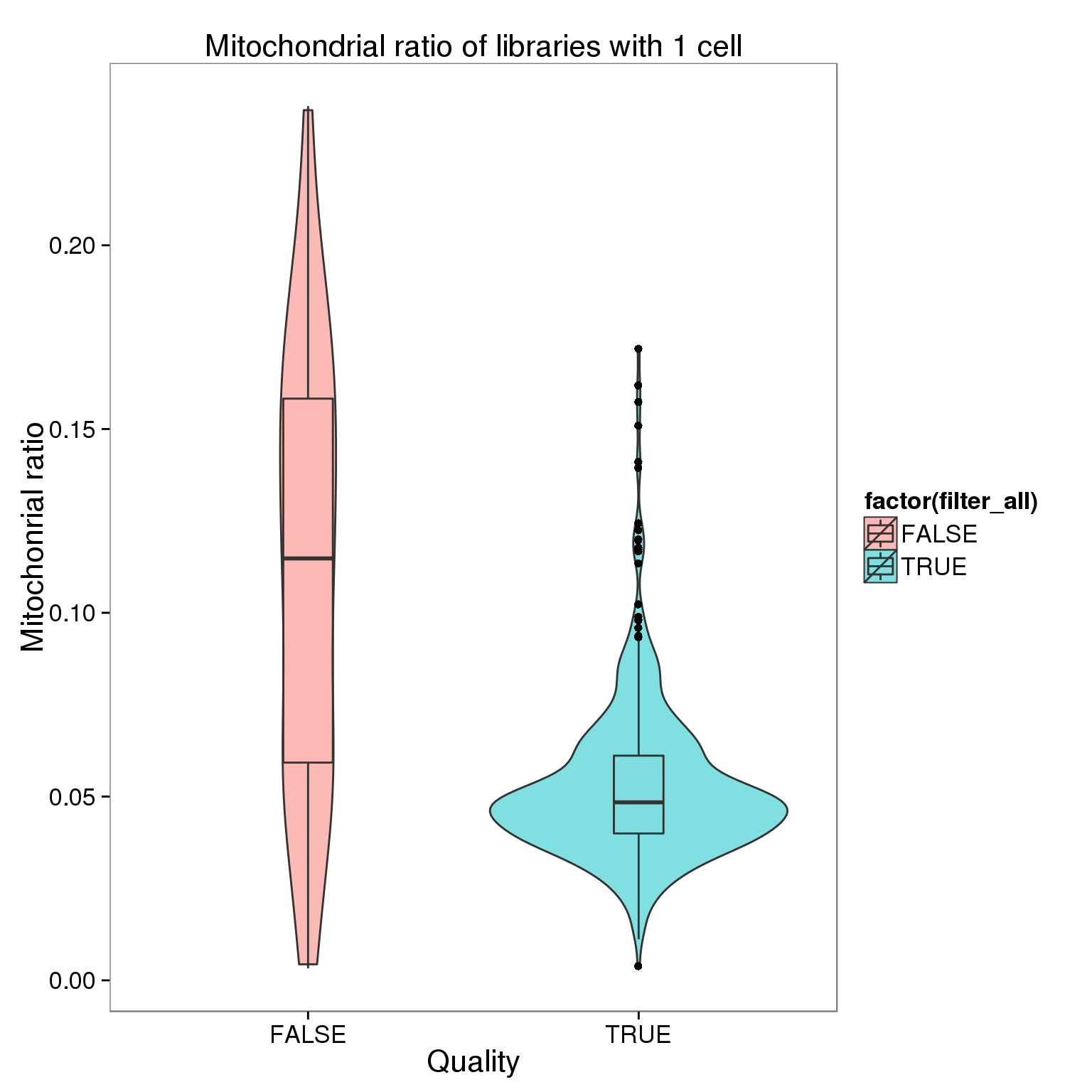
## check the batch of those outliers
mito_outliers <- summary_per_sample_reads_qc %>% filter(filter_all == "TRUE", mt_reads_ratio > .15)
mito_outliers  %>% dplyr::select(sample_id, mt_reads_ratio)
sample_id mt_reads_ratio
1 NA19098.r1.D07 0.1573689
2 NA19098.r3.G03 0.1618823
3 NA19098.r3.G04 0.1508871
4 NA19101.r3.A09 0.1718202## check if 19098 have high mt genes
ggplot(summary_per_sample_reads_qc[summary_per_sample_reads_qc$filter_all == "TRUE",],
aes(x = factor(batch), y = mt_reads_ratio,
fill = factor(batch)), height = 600, width = 2000) +
geom_violin(alpha = .5) +
geom_boxplot(alpha = .01, width = .2, position = position_dodge(width = .9)) +
scale_fill_manual(values = great_color_8) +
labs(x = "batch", y = "Mitochondrial ratio") +
theme(axis.text.x = element_text(hjust=1, angle = 45))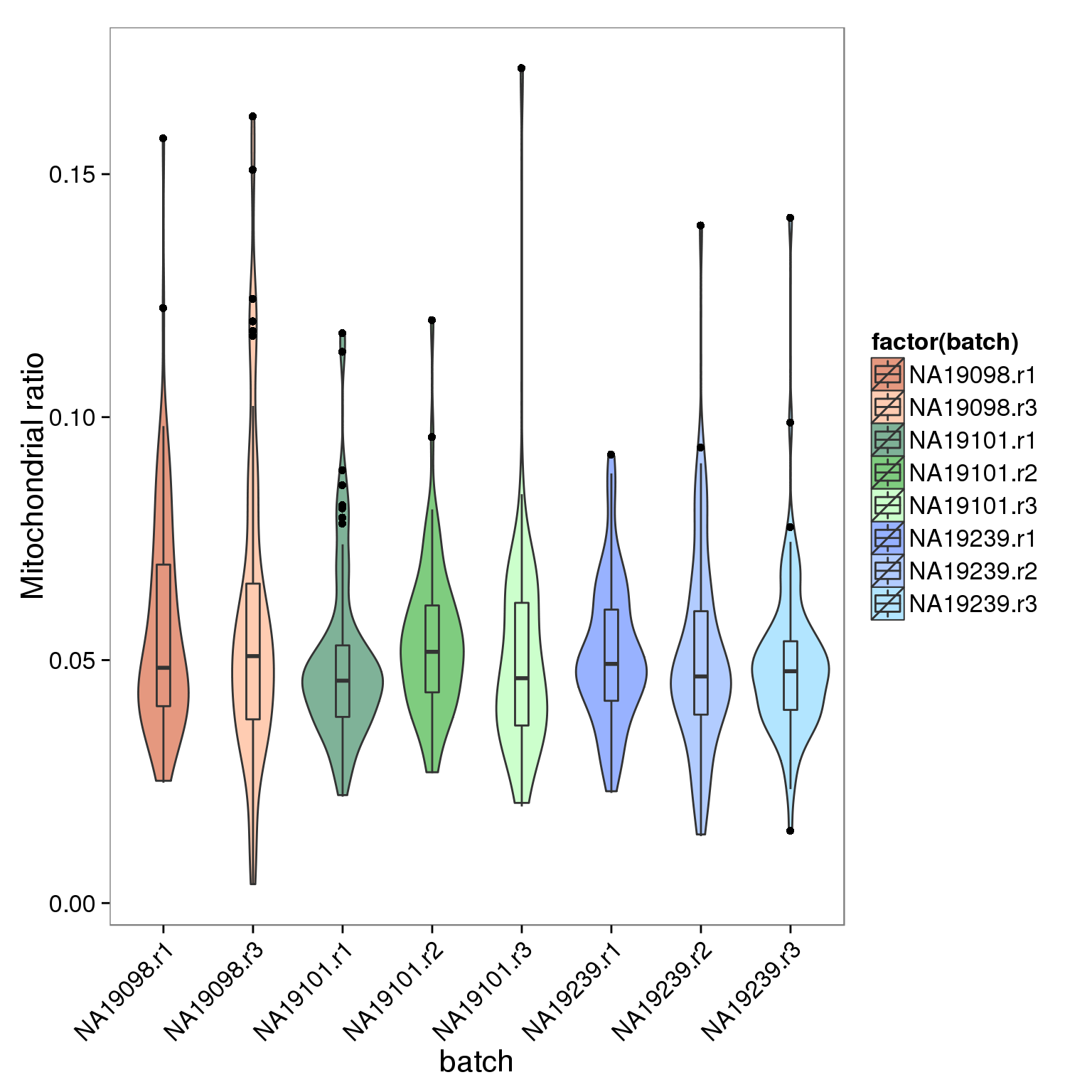
plots
genes_unmapped <-  ggplot(summary_per_sample_reads_qc,
                   aes(x = gene_number, y = unmapped_ratios * 100,
                   col = as.factor(individual), height = 600, width = 2000)) +
                   geom_point(size = 3, alpha = 0.3) +
                   geom_vline(xintercept = cut_off_genes, colour="grey", linetype = "longdash") +
                   geom_hline(yintercept = cut_off_unmapped * 100, colour="grey", linetype = "longdash") +
                   labs(x = "Number of detected genes / sample",
                        y = "Percentage of unmapped reads in each sample (%)",
                        title = "Number of genes detected as \n expressed as a function of \n the proportion of mapped reads")

genes_ercc <-  ggplot(summary_per_sample_reads_qc,
                   aes(x = gene_number, y = ercc_percentage * 100,
                   col = as.factor(individual), shape = as.factor(replicate), height = 600, width = 2000)) +
                   geom_point(size = 3, alpha = 0.3) +
                   geom_vline(xintercept = cut_off_genes, colour="grey", linetype = "longdash") +
                   geom_hline(yintercept = cut_off_ercc * 100, colour="grey", linetype = "longdash") +
                   labs(x = "Number of detected genes / samlpe",
                        y = "Percentage of ERCC reads in each sample (%)",
                        title = "Samples with zero cell \n (visual inspection) have \n low number of reads")

reads_unmapped_num <-  ggplot(summary_per_sample_reads_qc,
                   aes(x = total_mapped, y = unmapped_ratios * 100,
                   col = as.factor(individual), label = as.character(cell_number), height = 600, width = 2000)) +
                   geom_text(fontface = 3, alpha = 0.5) +
                   geom_vline(xintercept = cut_off_reads, colour="grey", linetype = "longdash") +
                   geom_hline(yintercept = cut_off_unmapped * 100, colour="grey", linetype = "longdash") +
                   labs(x = "Total mapped reads / sample",
                        y = "Percentage of unmapped reads in each sample (%)",
                        title = "Samples with zero cells \n (visual inspection) have \n high proportion of unmapped reads")

reads_ercc_num <-  ggplot(summary_per_sample_reads_qc,
                   aes(x = total_mapped, y = ercc_percentage * 100,
                   col = as.factor(individual), label = as.character(cell_number), height = 600, width = 2000)) +
                   geom_text(fontface = 3, alpha = 0.5) +
                   geom_vline(xintercept = cut_off_reads, colour="grey", linetype = "longdash") +
                   geom_hline(yintercept = cut_off_ercc * 100, colour="grey", linetype = "longdash") +
                   labs(x = "Total mapped reads / sample",
                        y = "Percentage of ERCC reads in each sample (%)",
                        title = "Samples with zero cells \n (visual inspection) have \n high proportion of ERCC reads")

plot_grid(genes_unmapped + theme(legend.position = "none"),
          genes_ercc + theme(legend.position = "none"),
          reads_unmapped_num + theme(legend.position = "none"),
          reads_ercc_num + theme(legend.position = "none"),
          labels = letters[1:4])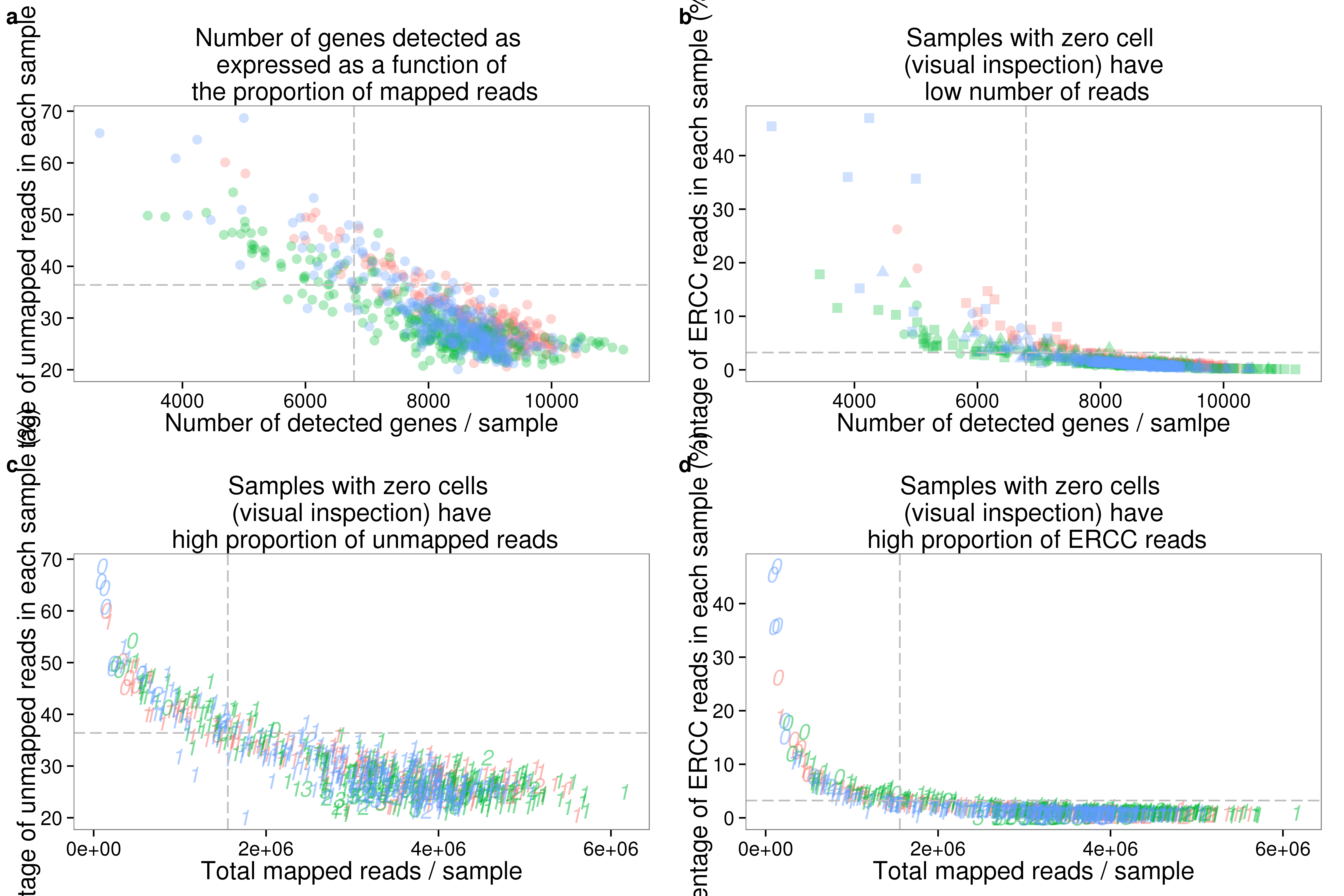
plot_grid(genes_unmapped + theme(legend.position = c(.75,.9)) + labs(col = "Individual"),
          reads_unmapped_num + theme(legend.position = "none"),
          reads_ercc_num + theme(legend.position = "none"),
          labels = letters[3:5],
          nrow = 1)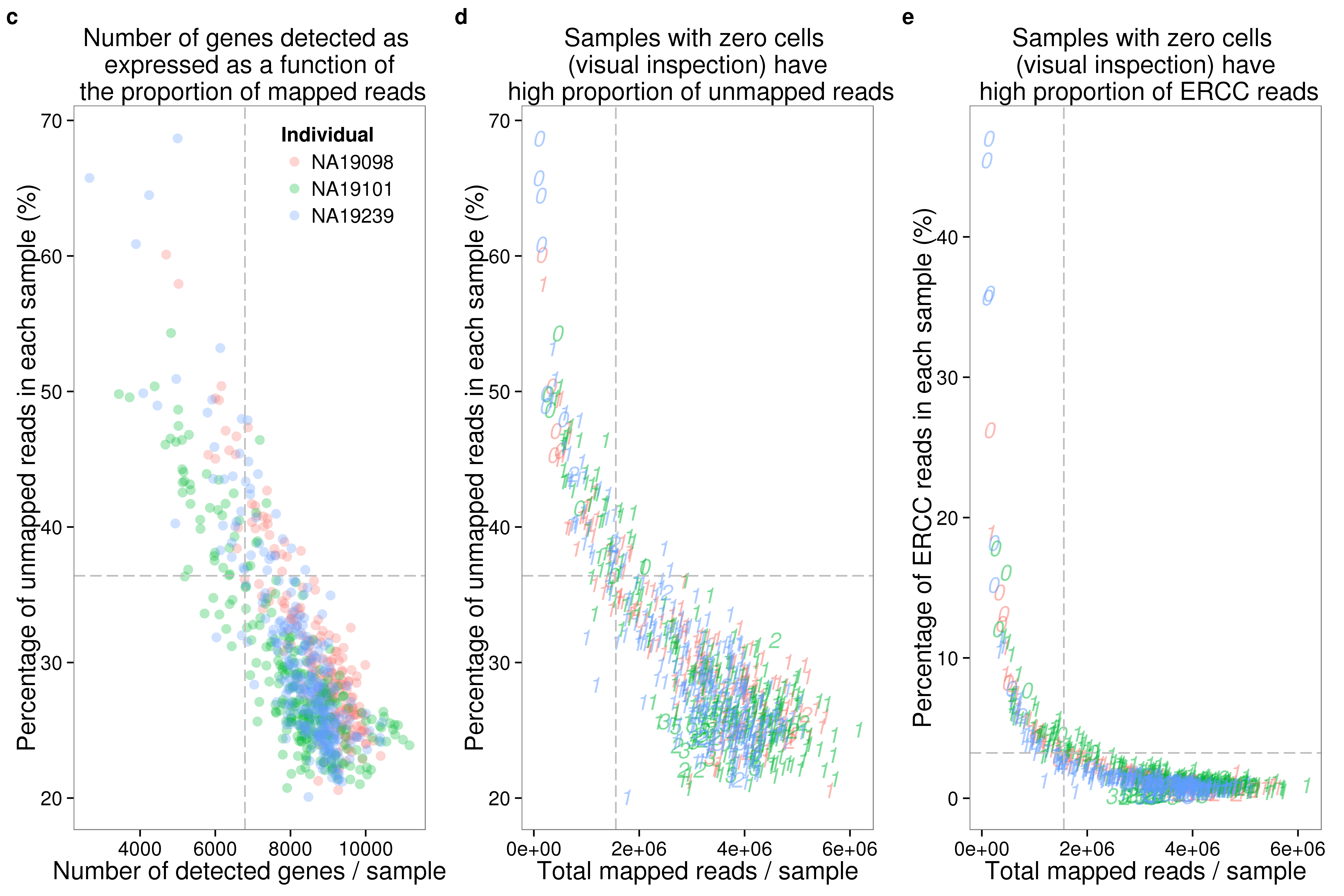
plot_grid(ercc_reads_plot + theme(legend.position = "none"),
          ercc_molecule_plot + theme(legend.position = "none"),
          plot_reads + theme(legend.position=c(.8,.85)),
          plot_unmapped + theme(legend.position = "none"),
          plot_ercc + theme(legend.position = "none"),
          plot_gene + theme(legend.position = "none"),
          labels = letters[1:6],
          ncol = 2)
plot_grid(plot_before + theme(legend.position=c(.85,.85)) + labs(col = "Cell number"),
          plot_after + theme(legend.position = "none"),
          plot_ercc_before,
          plot_ercc_after,
          labels = letters[1:4])
Session information
sessionInfo()R version 3.2.0 (2015-04-16)
Platform: x86_64-unknown-linux-gnu (64-bit)
locale:
[1] LC_CTYPE=en_US.UTF-8 LC_NUMERIC=C
[3] LC_TIME=en_US.UTF-8 LC_COLLATE=en_US.UTF-8
[5] LC_MONETARY=en_US.UTF-8 LC_MESSAGES=en_US.UTF-8
[7] LC_PAPER=en_US.UTF-8 LC_NAME=C
[9] LC_ADDRESS=C LC_TELEPHONE=C
[11] LC_MEASUREMENT=en_US.UTF-8 LC_IDENTIFICATION=C
attached base packages:
[1] stats graphics grDevices utils datasets methods base
other attached packages:
[1] MASS_7.3-40 cowplot_0.3.1 ggplot2_1.0.1 edgeR_3.10.2 limma_3.24.9
[6] dplyr_0.4.2 knitr_1.10.5
loaded via a namespace (and not attached):
[1] Rcpp_0.12.4 magrittr_1.5 munsell_0.4.3
[4] colorspace_1.2-6 R6_2.1.1 stringr_1.0.0
[7] httr_0.6.1 plyr_1.8.3 tools_3.2.0
[10] parallel_3.2.0 grid_3.2.0 gtable_0.1.2
[13] DBI_0.3.1 htmltools_0.2.6 lazyeval_0.1.10
[16] yaml_2.1.13 assertthat_0.1 digest_0.6.8
[19] RColorBrewer_1.1-2 reshape2_1.4.1 formatR_1.2
[22] bitops_1.0-6 RCurl_1.95-4.6 evaluate_0.7
[25] rmarkdown_0.6.1 labeling_0.3 stringi_1.0-1
[28] scales_0.4.0 proto_0.3-10