Compare high/low-CV genes between individuals
Joyce Hsiao
2015-10-26
Last updated: 2015-12-11
Code version: a795f9edad85aa99750bd8425fbe4d89346cfd42
Objective
Based on the data filtered of PC1, we computed CVs of each individual and identified genes of high/low coefficients of variation.
Set up
library("data.table")
library("dplyr")
library("limma")
library("edgeR")
library("ggplot2")
library("grid")
theme_set(theme_bw(base_size = 12))
source("functions.R")
Prepare data
Input annotation of only QC-filtered single cells. Remove NA19098.r2
anno_qc_filter <- read.table("../data/annotation-filter.txt", header = TRUE,
                   stringsAsFactors = FALSE)
Import endogeneous gene molecule counts that are QC-filtered, CPM-normalized, ERCC-normalized, and also processed to remove unwanted variation from batch effet. ERCC genes are removed from this file.
molecules_ENSG <- read.table("../data/molecules-final.txt", header = TRUE, stringsAsFactors = FALSE)Input moleclule counts before log2 CPM transformation. This file is used to compute percent zero-count cells per sample.
molecules_sparse <- read.table("../data/molecules-filter.txt", header = TRUE, stringsAsFactors = FALSE)

molecules_sparse <- molecules_sparse[grep("ENSG", rownames(molecules_sparse)), ]
stopifnot( all.equal(rownames(molecules_ENSG), rownames(molecules_sparse)) )
Remove the first PC
library(matrixStats)
centered_ENSG <- molecules_ENSG - rowMeans(molecules_ENSG)
svd_all <- svd( centered_ENSG )
filtered_data <- with(svd_all, u %*% diag( c(0, d[-1]) ) %*% t(v))
Compute CV of the filtered data
cv_filtered <- lapply(1:3, function(ii_individual) {
    individuals <- unique(anno_qc_filter$individual)
    counts <- filtered_data[ , anno_qc_filter$individual == individuals [ii_individual]]
    means <- apply(counts, 1, mean)
    sds <- apply(counts, 1, sd)
    cv <- sds/means
    return(cv)
})
names(cv_filtered) <- unique(anno_qc_filter$individual)
cv_filtered <- do.call(cbind, cv_filtered)
Plot CVs between indivdiuals
par(mfrow = c(2,2))
plot(x = cv_filtered[,1], y = cv_filtered[,2], pch = 16, cex = .6)
plot(x = cv_filtered[,3], y = cv_filtered[,2], pch = 16, cex = .6)
plot(x = cv_filtered[,1], y = cv_filtered[,3], pch = 16, cex = .6)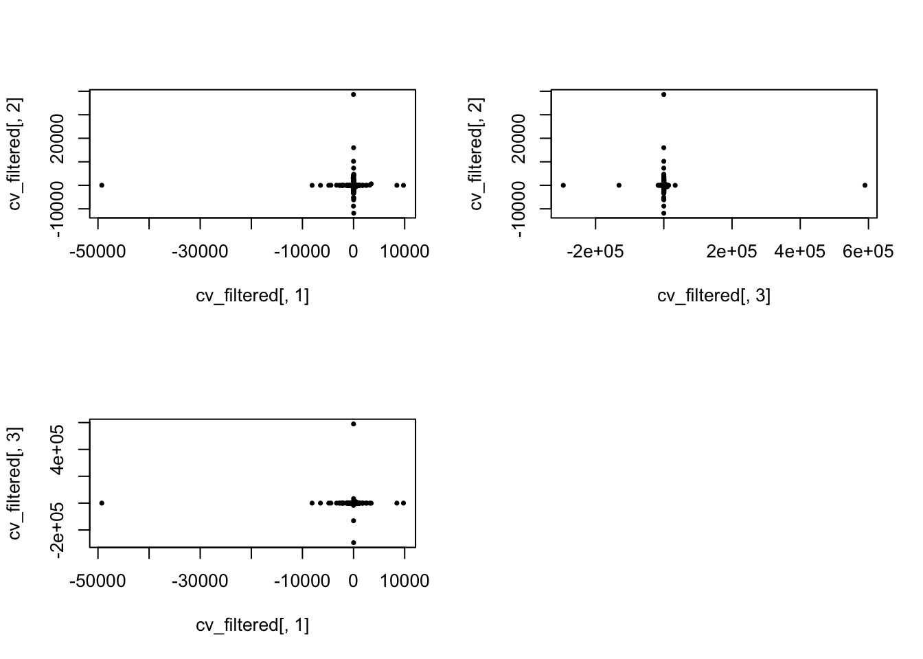
High CVs
No genes with CV high in all individuals.
means_cv <- mean(unlist(cv_filtered))
sds_cv <- sd(unlist(cv_filtered))
ii_high_2 <- lapply(1:3, function(ii_individual) {
                which(cv_filtered[ ,ii_individual] > means_cv + 2*sds_cv) })
length(Reduce(intersect, ii_high_2))
[1] 0length(Reduce(union, ii_high_2))[1] 14ii_high_all <- Reduce(union, ii_high_2)
par(mfrow = c(2,2))
plot(x = cv_filtered[,1], y = cv_filtered[,2], pch = 16, cex = .6,
xlim = c(0, max(cv_filtered[,1])), ylim = c(0, max(cv_filtered[,2])))
points(x = cv_filtered[ii_high_all, 1],
y = cv_filtered[ii_high_all, 2], pch = 1, cex = .8, col = "red")
plot(x = cv_filtered[,3], y = cv_filtered[,2], pch = 16, cex = .6,
xlim = c(0, max(cv_filtered[,3])), ylim = c(0, max(cv_filtered[,2])))
points(x = cv_filtered[ii_high_all, 3],
y = cv_filtered[ii_high_all, 2], pch = 1, cex = .8, col = "red")
plot(x = cv_filtered[,1], y = cv_filtered[,3], pch = 16, cex = .6,
xlim = c(0, max(cv_filtered[,1])), ylim = c(0, max(cv_filtered[,3])))
points(x = cv_filtered[ii_high_all, 1],
y = cv_filtered[ii_high_all, 3], pch = 1, cex = .8, col = "red")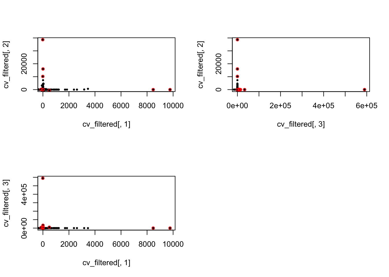
Outliers..
par(mfrow = c(2,2))
plot(density(filtered_data[ which.max(cv_filtered[,1]),
                            anno_qc_filter$individual == "NA19098"]))
plot(density(filtered_data[ which.max(cv_filtered[,2]),
                            anno_qc_filter$individual == "NA19101"]))
plot(density(filtered_data[ which.max(cv_filtered[,3]),
                            anno_qc_filter$individual == "NA19239"]))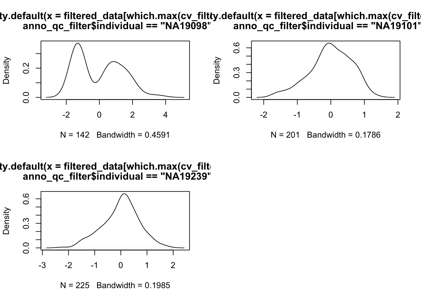
Low CVs
No genes with CV high in all individuals.
means_cv <- mean(unlist(cv_filtered))
sds_cv <- sd(unlist(cv_filtered))
ii_low_2 <- lapply(1:3, function(ii_individual) {
                which(cv_filtered[ ,ii_individual] < means_cv - 2*sds_cv) })
length(Reduce(intersect, ii_low_2))
[1] 0length(Reduce(union, ii_low_2))[1] 11ii_low_all <- Reduce(union, ii_low_2)
par(mfrow = c(2,2))
plot(x = cv_filtered[,1], y = cv_filtered[,2], pch = 16, cex = .6,
xlim = c(0, max(cv_filtered[,1])), ylim = c(0, max(cv_filtered[,2])))
points(x = cv_filtered[ii_low_all, 1],
y = cv_filtered[ii_low_all, 2], pch = 1, cex = .8, col = "red")
plot(x = cv_filtered[,3], y = cv_filtered[,2], pch = 16, cex = .6,
xlim = c(0, max(cv_filtered[,3])), ylim = c(0, max(cv_filtered[,2])))
points(x = cv_filtered[ii_low_all, 3],
y = cv_filtered[ii_low_all, 2], pch = 1, cex = .8, col = "red")
plot(x = cv_filtered[,1], y = cv_filtered[,3], pch = 16, cex = .6,
xlim = c(0, max(cv_filtered[,1])), ylim = c(0, max(cv_filtered[,3])))
points(x = cv_filtered[ii_low_all, 1],
y = cv_filtered[ii_low_all, 3], pch = 1, cex = .8, col = "red")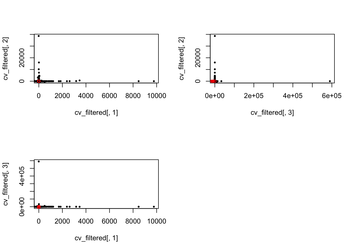
Outliers..
par(mfrow = c(2,2))
plot(density(filtered_data[ which.min(cv_filtered[,1]),
                            anno_qc_filter$individual == "NA19098"]))
plot(density(filtered_data[ which.min(cv_filtered[,2]),
                            anno_qc_filter$individual == "NA19101"]))
plot(density(filtered_data[ which.min(cv_filtered[,3]),
                            anno_qc_filter$individual == "NA19239"]))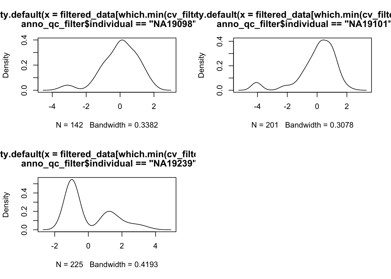
Why CVs are orthogonal between individuals??
Compute CV before filtering PC1
cv_data <- lapply(1:3, function(ii_individual) {
    individuals <- unique(anno_qc_filter$individual)
    counts <- molecules_ENSG[ , anno_qc_filter$individual == individuals [ii_individual]]
    means <- apply(counts, 1, mean)
    sds <- apply(counts, 1, sd)
    cv <- sds/means
    return(cv)
})
names(cv_data) <- unique(anno_qc_filter$individual)
cv_data <- do.call(cbind, cv_data)

par(mfrow = c(2,2))
plot(x = cv_data[,1], y = cv_data[,2], pch = 16, cex = .6,
     xlim = c(0, 1), ylim = c(0, 1))
plot(x = cv_data[,3], y = cv_data[,2], pch = 16, cex = .6,
     xlim = c(0, 1), ylim = c(0, 1))
plot(x = cv_data[,1], y = cv_data[,3], pch = 16, cex = .6,
     xlim = c(0, 1), ylim = c(0, 1))
title(main = "CV before PC1 removal", outer = TRUE, line = -1)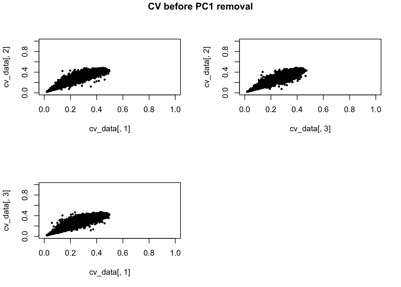
Mean gene expression level before removing PC1.
means_data <- lapply(1:3, function(ii_individual) {
    individuals <- unique(anno_qc_filter$individual)
    counts <- molecules_ENSG[ , anno_qc_filter$individual == individuals [ii_individual]]
    means <- apply(counts, 1, mean)
    return(means)
})
names(means_data) <- unique(anno_qc_filter$individual)
means_data <- do.call(cbind, means_data)

par(mfrow = c(2,2))
plot(x = means_data[,1], y = means_data[,2], pch = 16, cex = .6)
plot(x = means_data[,3], y = means_data[,2], pch = 16, cex = .6)
plot(x = means_data[,1], y = means_data[,3], pch = 16, cex = .6)
title(main = "Means before PC1 removal", outer = TRUE, line = -1)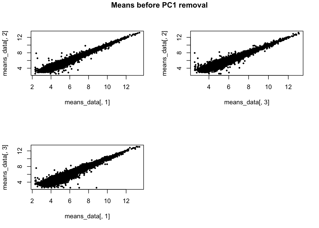
GO analysis
High CV
if (file.exists("rda/svd-filtered-high-low/go-high.rda")) {
load("rda/svd-filtered-high-low/go-high.rda")
} else {
library(Humanzee)
go_high <- lapply(1: 3, function(ii_individual) {
go_list <- GOtest(my_ensembl_gene_universe = rownames(molecules_ENSG),
my_ensembl_gene_test = rownames(molecules_ENSG)[ii_high_2[[ii_individual]]],
pval_cutoff = 1, ontology=c("BP","CC","MF") )
# Biological process
goterms_bp <- summary(go_list$GO$BP, pvalue = 1)
goterms_bp <- data.frame(ID = goterms_bp[[1]],
Pvalue = goterms_bp[[2]],
Terms = goterms_bp[[7]])
goterms_bp <- goterms_bp[order(goterms_bp$Pvalue), ]
# Cellular component
goterms_cc <- summary(go_list$GO$CC, pvalue = 1)
goterms_cc <- data.frame(ID = goterms_cc[[1]],
Pvalue = goterms_cc[[2]],
Terms = goterms_cc[[7]])
goterms_cc <- goterms_cc[order(goterms_cc$Pvalue), ]
# Molecular function
goterms_mf <- summary(go_list$GO$MF, pvalue = 1)
goterms_mf <- data.frame(ID = goterms_mf[[1]],
Pvalue = goterms_mf[[2]],
Terms = goterms_mf[[7]])
goterms_mf <- goterms_mf[order(goterms_mf$Pvalue), ]
return(list(goterms_bp = goterms_bp,
goterms_cc = goterms_cc,
goterms_mf = goterms_mf))
})
save(go_high, file = "rda/svd-filtered-high-low/go-high.rda")
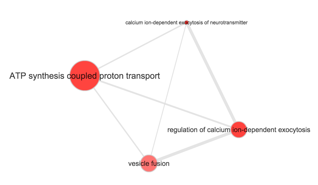
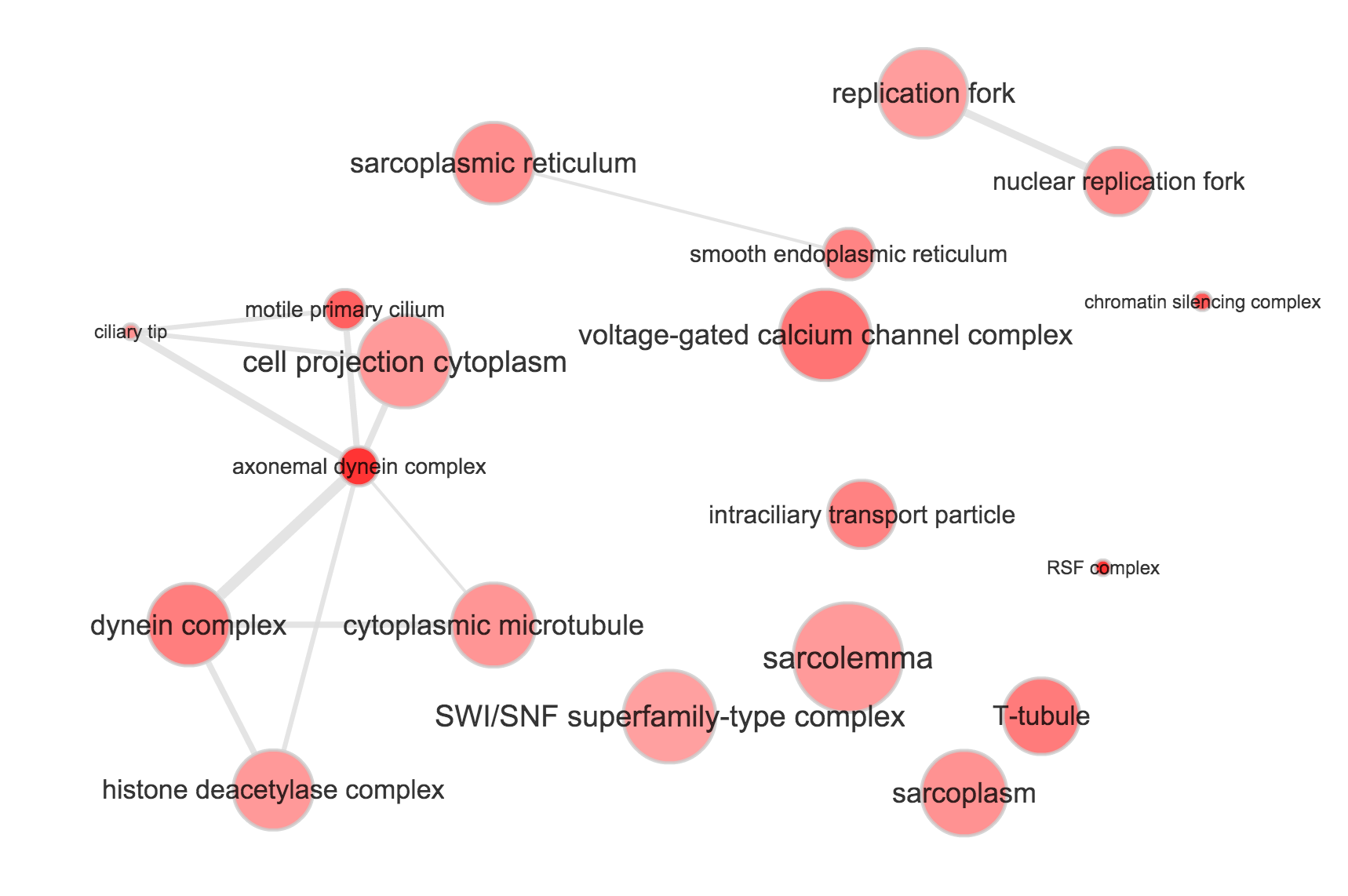
}Use REVIGO to summarize and visualize GO terms…
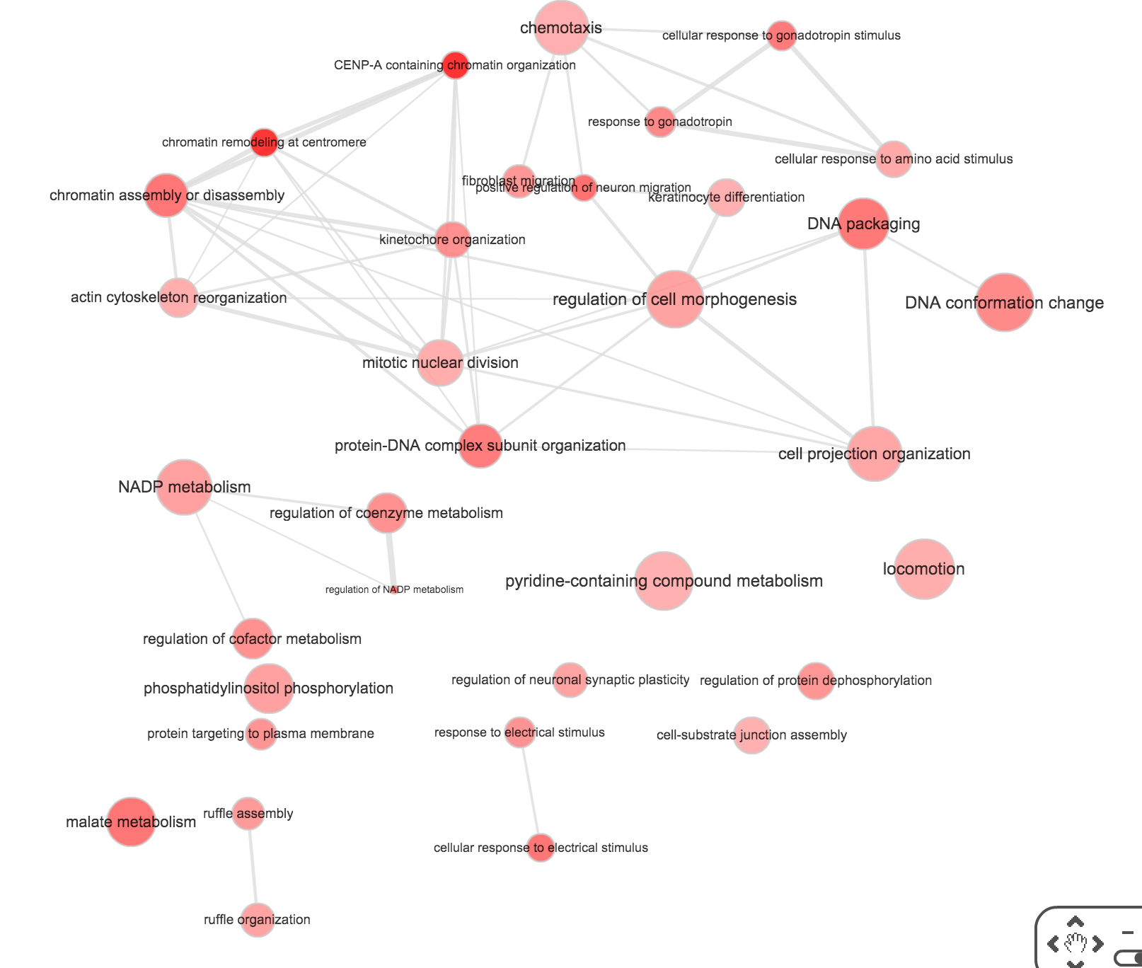
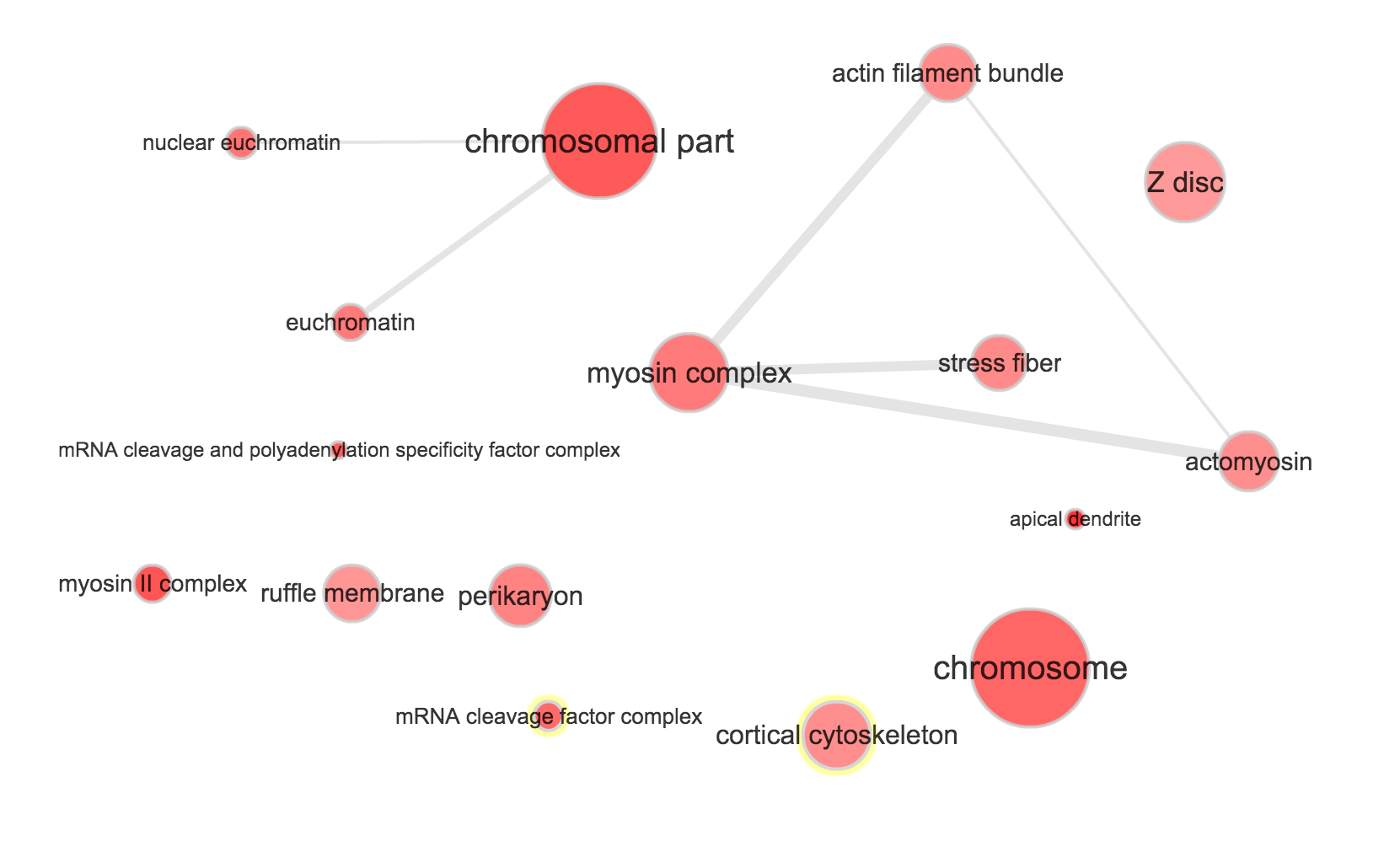
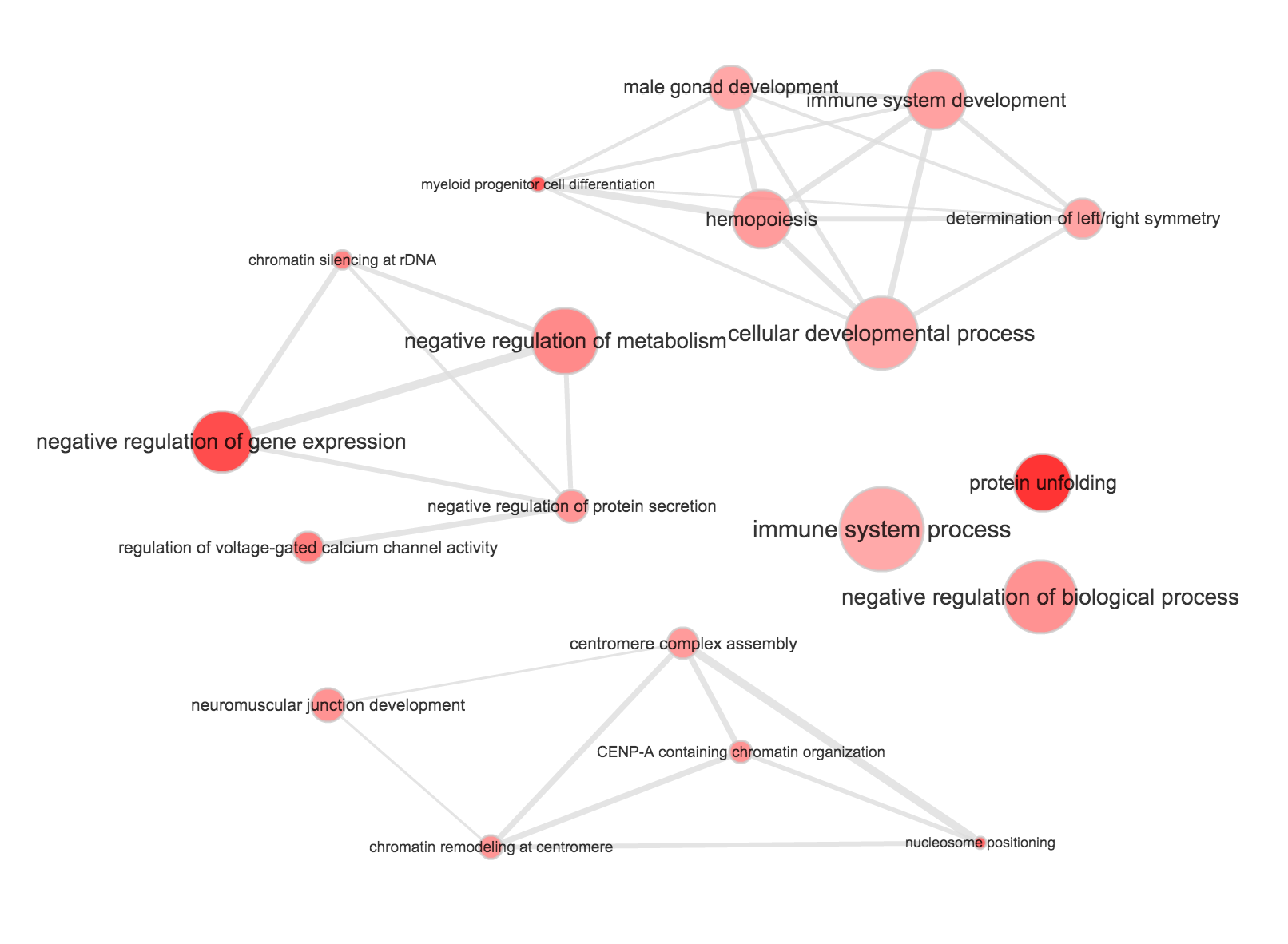
The size of the node indicates the p-vlaue of the GO term. The width of the edges indicates degree of similarity between the GO terms.
NA19098
- Biological process
- Cellular component
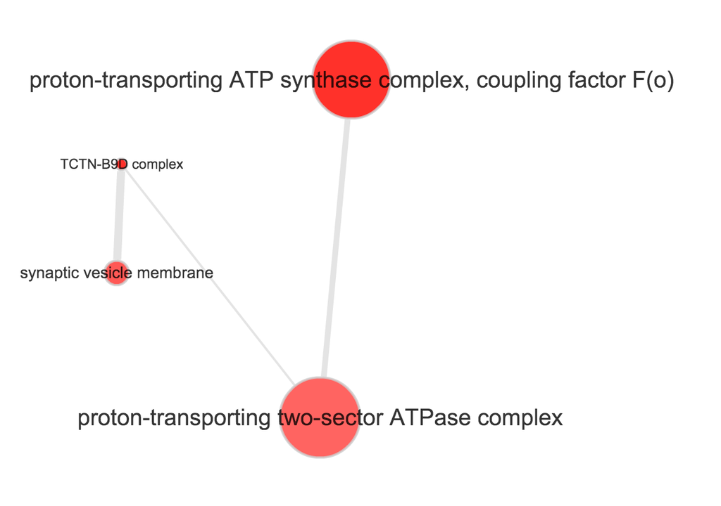
- Molecular function
NA19101
- Biological process
- Cellular component
- Molecular function
NA19239
- Biological process
- Cellular component
- Molecular function
Low CV
if (file.exists("rda/svd-filtered-high-low/go-low.rda")) {
  load("rda/svd-filtered-high-low/go-low.rda")
} else {
library(Humanzee)
go_low <- lapply(1: 3, function(ii_individual) {

  go_list <- GOtest(my_ensembl_gene_universe = rownames(molecules_ENSG),
                    my_ensembl_gene_test = rownames(molecules_ENSG)[ii_low_2[[ii_individual]]],
                    pval_cutoff = 1, ontology=c("BP","CC","MF") )

  # Biological process
  goterms_bp <- summary(go_list$GO$BP, pvalue = 1)
  goterms_bp <- data.frame(ID = goterms_bp[[1]],
                           Pvalue = goterms_bp[[2]],
                           Terms = goterms_bp[[7]])
  goterms_bp <- goterms_bp[order(goterms_bp$Pvalue), ]

  # Cellular component
  goterms_cc <- summary(go_list$GO$CC, pvalue = 1)
  goterms_cc <- data.frame(ID = goterms_cc[[1]],
                           Pvalue = goterms_cc[[2]],
                           Terms = goterms_cc[[7]])
  goterms_cc <- goterms_cc[order(goterms_cc$Pvalue), ]

  # Molecular function
  goterms_mf <- summary(go_list$GO$MF, pvalue = 1)
  goterms_mf <- data.frame(ID = goterms_mf[[1]],
                           Pvalue = goterms_mf[[2]],
                           Terms = goterms_mf[[7]])
  goterms_mf <- goterms_mf[order(goterms_mf$Pvalue), ]

  return(list(goterms_bp = goterms_bp,
              goterms_cc = goterms_cc,
              goterms_mf = goterms_mf))
})
  save(go_low, file = "rda/svd-filtered-high-low/go-low.rda")
}
Session information
sessionInfo()R version 3.2.1 (2015-06-18)
Platform: x86_64-apple-darwin13.4.0 (64-bit)
Running under: OS X 10.10.5 (Yosemite)
locale:
[1] en_US.UTF-8/en_US.UTF-8/en_US.UTF-8/C/en_US.UTF-8/en_US.UTF-8
attached base packages:
[1] grid stats graphics grDevices utils datasets methods
[8] base
other attached packages:
[1] matrixStats_0.15.0 ggplot2_1.0.1 edgeR_3.10.5
[4] limma_3.24.15 dplyr_0.4.3 data.table_1.9.6
[7] knitr_1.11
loaded via a namespace (and not attached):
[1] Rcpp_0.12.2 magrittr_1.5 MASS_7.3-45 munsell_0.4.2
[5] colorspace_1.2-6 R6_2.1.1 stringr_1.0.0 plyr_1.8.3
[9] tools_3.2.1 parallel_3.2.1 gtable_0.1.2 DBI_0.3.1
[13] htmltools_0.2.6 yaml_2.1.13 assertthat_0.1 digest_0.6.8
[17] reshape2_1.4.1 formatR_1.2.1 evaluate_0.8 rmarkdown_0.8.1
[21] stringi_1.0-1 scales_0.3.0 chron_2.3-47 proto_0.3-10