Total molecule counts
Po-Yuan Tung
2016-04-18
Last updated: 2016-11-08
Code version: bd286a36f14d3b332285cdc7e62258b1f616bb14
Recreate the Sequencing depth and cellular RNA content using updated data files to make figures for the paper.
Setup
library("dplyr")
library("tidyr")
library("edgeR")
library("lmtest")
library("ggplot2")
library("cowplot")
theme_set(theme_bw(base_size = 16))
theme_update(panel.grid.minor.x = element_blank(),
             panel.grid.minor.y = element_blank(),
             panel.grid.major.x = element_blank(),
             panel.grid.major.y = element_blank(),
             legend.key = element_blank(),
             plot.title = element_text(size = rel(1)))
source("functions.R")
Input annotation
anno_single <- read.table("../data/annotation.txt", header = TRUE,
                   stringsAsFactors = FALSE)
head(anno_single)
individual replicate well batch sample_id
1 NA19098 r1 A01 NA19098.r1 NA19098.r1.A01
2 NA19098 r1 A02 NA19098.r1 NA19098.r1.A02
3 NA19098 r1 A03 NA19098.r1 NA19098.r1.A03
4 NA19098 r1 A04 NA19098.r1 NA19098.r1.A04
5 NA19098 r1 A05 NA19098.r1 NA19098.r1.A05
6 NA19098 r1 A06 NA19098.r1 NA19098.r1.A06Input single cell observational quality control data.
qc <- read.table("../data/qc-ipsc.txt", header = TRUE,
                 stringsAsFactors = FALSE)
qc <- qc %>% arrange(individual, replicate, well)
stopifnot(qc$individual == anno_single$individual,
          qc$replicate == anno_single$replicate,
          qc$well == anno_single$well)
head(qc)
individual replicate well cell_number concentration tra1.60
1 NA19098 r1 A01 1 1.734785 1
2 NA19098 r1 A02 1 1.723038 1
3 NA19098 r1 A03 1 1.512786 1
4 NA19098 r1 A04 1 1.347492 1
5 NA19098 r1 A05 1 2.313047 1
6 NA19098 r1 A06 1 2.056803 1Incorporate informatin on cell number, concentration, and TRA1-60 status.
anno_single$cell_number <- qc$cell_number
anno_single$concentration <- qc$concentration
anno_single$tra1.60 <- qc$tra1.60
Keep only quality single cell
quality_single_cells <- scan("../data/quality-single-cells.txt",
                             what = "character")
anno_single <- anno_single[anno_single$sample_id %in% quality_single_cells,]
Input molecule counts after filtering
molecules <- read.table("../data/molecules-filter.txt", header = TRUE,
                    stringsAsFactors = FALSE)
stopifnot(colnames(molecules) == anno_single$sample_id)
ercc_index <- grepl("ERCC", rownames(molecules))
anno_single$total_molecules_gene = colSums(molecules[!ercc_index, ])
anno_single$total_molecules_ercc = colSums(molecules[ercc_index, ])
anno_single$total_molecules = colSums(molecules)
anno_single$num_genes = apply(molecules[!ercc_index, ], 2, function(x) sum(x > 0))
The total molecule-counts
For wells with a single cell observed, the total molecule-counts range from 30408 to 113832, the first quartile for the total number of gene molecules is 55561.25, and the third quartile is 78173.25.
## create a color palette with one color per individual and different shades for repplicates
great_color_8 <- c("#CC3300", "#FF9966", "#006633", "#009900", "#99FF99", "#3366FF", "#6699FF", "#66CCFF")

plot_total_molecules_gene <- ggplot(anno_single,
                       aes(x = as.factor(batch), y = total_molecules_gene / 10^3, fill = as.factor(batch))) +
                       geom_boxplot(alpha = .01, width = .2) +
                       geom_violin(alpha = .5) +
                       scale_fill_manual(values = great_color_8) +
                       labs(x = "Batch", y = "Total gene molecule-counts (10^3)",
                            title = "Total gene molecule-counts are affected \n by individual and technical C1 batch") +
                       theme(axis.text.x = element_text(hjust=1, angle = 45))

plot_total_molecules_ercc <-  plot_total_molecules_gene %+%
                                   aes(y = total_molecules_ercc / 10^3) +
                                   labs(y = "Total ERCC molecule-counts (10^3)",
                                        title = "Total ERCC molecule-counts are affected \n by individual and technical C1 batch")

summary(aov(total_molecules_gene ~ individual, data = anno_single))
Df Sum Sq Mean Sq F value Pr(>F)
individual 2 2.571e+10 1.286e+10 70.39 <2e-16 ***
Residuals 561 1.025e+11 1.827e+08
---
Signif. codes: 0 '***' 0.001 '**' 0.01 '*' 0.05 '.' 0.1 ' ' 1plot_grid(plot_total_molecules_gene + theme(legend.position = "none"),
plot_total_molecules_ercc + theme(legend.position = "none"),
labels = LETTERS[1:2])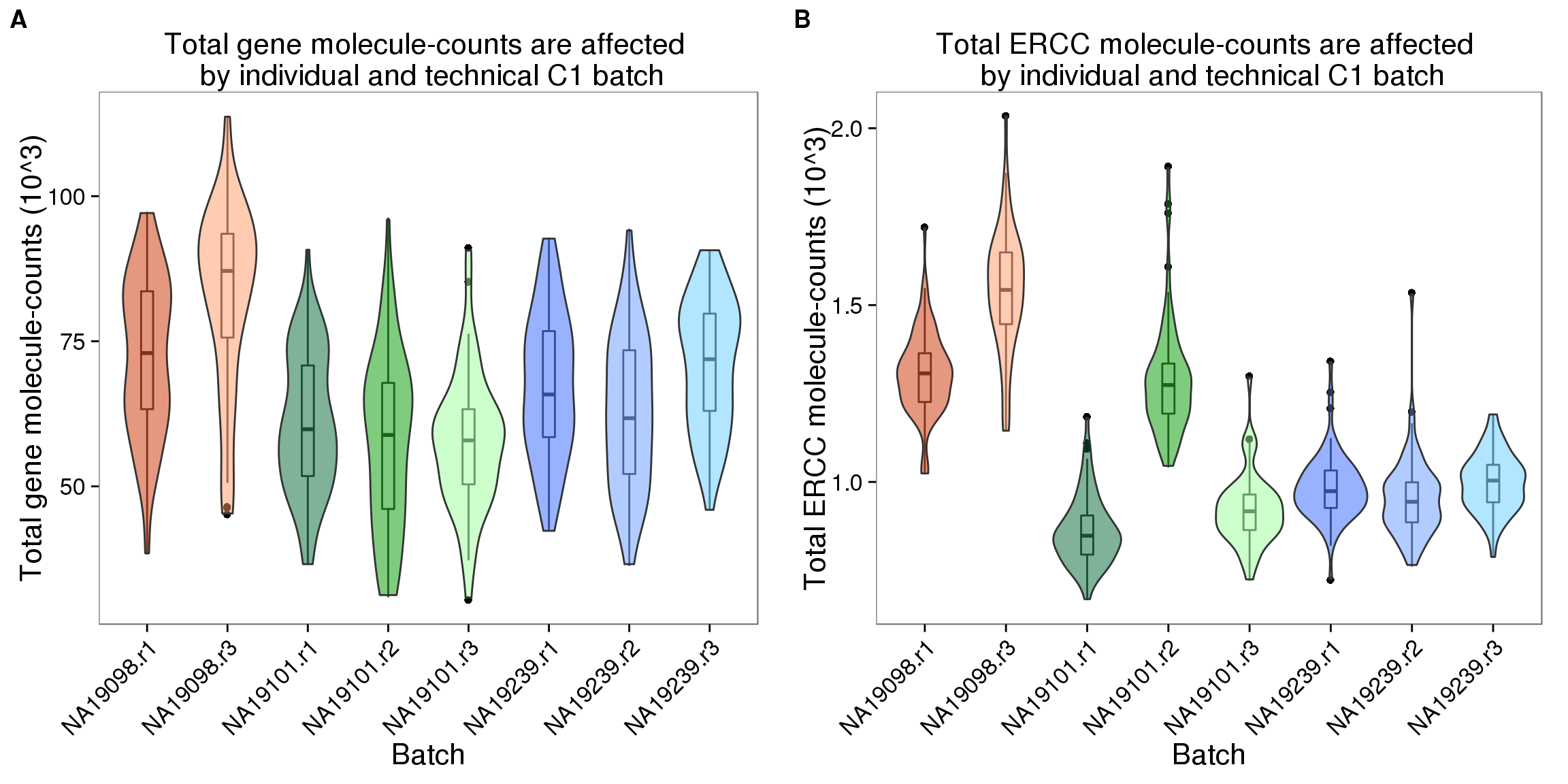
The relationship between concentration and total molecule-counts (not including NA19098)
As we try to understand the general relationships between sequencing results and cellular mRNA content, we remove outlier batches. NA19098 replicate 1 failed the quantification of the concentration of the single cells and was hence removed. Because NA19098 concentration is only quantified in one replicate, we removed NA19098 from analysis involving batch differences and concentration.
anno_single_6 <- anno_single %>% filter(individual != "NA19098")## look at endogenous genes
plot_conc_molecules_gene_individual <-
ggplot(anno_single_6,
aes(x = concentration,
y = total_molecules_gene / 10^3, color = individual)) +
geom_point(alpha = 0.8) +
scale_colour_manual(values = c("#33CC66", "#6699FF")) +
geom_smooth(method = "lm", se = FALSE) +
labs(x = "Concentration (ng/ul)", y = "Total gene molecule-counts (10^3)")
## look at ERCC spike-ins
plot_conc_molecules_ercc_individual <-
plot_conc_molecules_gene_individual %+%
aes(y = total_molecules_ercc / 10^3) +
labs(y = "Total ERCC molecule-counts (10^3)")
## plots
plot_grid(plot_conc_molecules_gene_individual + theme(legend.position = "none"),
plot_conc_molecules_ercc_individual + theme(legend.position = "none"),
labels = LETTERS[1:2])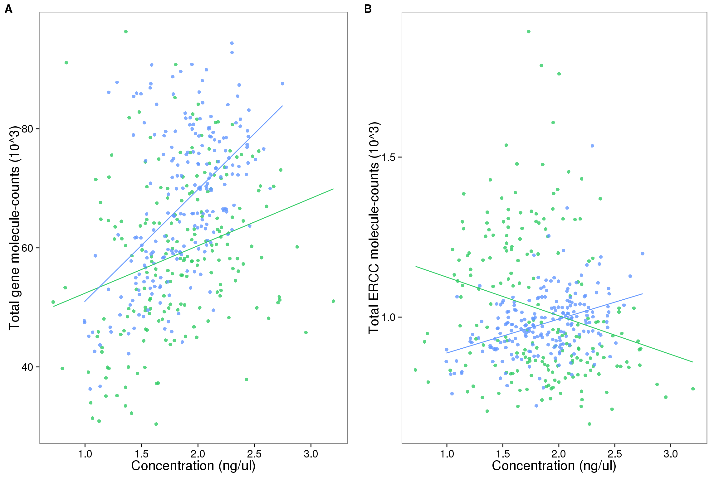
## Is there a difference across the three individuals
table(anno_single_6$individual, anno_single_6$replicate)
          r1 r2 r3
  NA19101 80 70 51
  NA19239 74 68 79
fit0 <- lm(total_molecules_gene ~ concentration,
data = anno_single_6)
fit1 <- lm(total_molecules_gene ~ concentration + as.factor(individual),
data = anno_single_6)
# use likelihood ratio test to detect individual differences
lrtest(fit1, fit0)Likelihood ratio test
Model 1: total_molecules_gene ~ concentration + as.factor(individual)
Model 2: total_molecules_gene ~ concentration
#Df LogLik Df Chisq Pr(>Chisq)
1 4 -4555.1
2 3 -4577.1 -1 43.956 3.358e-11 ***
---
Signif. codes: 0 '***' 0.001 '**' 0.01 '*' 0.05 '.' 0.1 ' ' 1Calculate correlation of concentration and molecule counts
## for each individual
for (i in 1:length(unique(anno_single_6$individual))) {
    print(unique(anno_single_6$individual)[i])
    select_individual <- with(anno_single_6, individual == unique(individual)[i])
    print(cor(anno_single_6[select_individual,7],anno_single_6[select_individual,9]))
}
[1] "NA19101"
[1] 0.2767428
[1] "NA19239"
[1] 0.524656## for each batch
for (i in 1:length(unique(anno_single_6$batch))) {
print(unique(anno_single_6$batch)[i])
select_replicate <- with(anno_single_6, batch == unique(batch)[i])
print(cor(anno_single_6[select_replicate,7],
anno_single_6[select_replicate,9]))
}[1] "NA19101.r1"
[1] 0.3607414
[1] "NA19101.r2"
[1] 0.5084765
[1] "NA19101.r3"
[1] -0.0631127
[1] "NA19239.r1"
[1] 0.7466212
[1] "NA19239.r2"
[1] 0.7784135
[1] "NA19239.r3"
[1] -0.03799184ERCC counts and total molecule counts
## calulate ERCC percentage
anno_single <- anno_single %>%
  mutate(perc_ercc_molecules = total_molecules_ercc / total_molecules * 100)

## ERCC molecule versus total molecule
plot_gene_mol_ercc_mol <- ggplot(anno_single,
                                 aes(x = total_molecules_gene,
                                     y = total_molecules_ercc)) +
                         geom_point(aes(color = individual, shape = replicate), alpha = 0.8)+
                         scale_shape(name = "Replicate")+
                         scale_color_discrete(name = "Individual")+
                         guides(color = guide_legend(order = 1),
                                shape = guide_legend(order = 2))+
                         labs(x = "Total gene molecule-counts per sample",
                              y = "Total ERCC molecule-counts per sample",
                              title = "The effect of individual and C1 batch on \n the correlation between total molecule-counts \n of endogenous genes and ERCC controls")

plot_gene_mol_perc_ercc <- plot_gene_mol_ercc_mol %+%
                           aes(x = perc_ercc_molecules)+
                           labs(x = "Percent ERCC molecules")

## Is there a difference across the three individuals
table(anno_single$individual, anno_single$replicate)
          r1 r2 r3
  NA19098 85  0 57
  NA19101 80 70 51
  NA19239 74 68 79
fit0 <- lm(total_molecules_ercc ~ 1, data = anno_single)
fit1 <- lm(total_molecules_ercc ~ 1 + as.factor(individual), data = anno_single)
anova(fit0, fit1)Analysis of Variance Table
Model 1: total_molecules_ercc ~ 1
Model 2: total_molecules_ercc ~ 1 + as.factor(individual)
Res.Df RSS Df Sum of Sq F Pr(>F)
1 563 34614165
2 561 17394891 2 17219274 277.67 < 2.2e-16 ***
---
Signif. codes: 0 '***' 0.001 '**' 0.01 '*' 0.05 '.' 0.1 ' ' 1## Is there a difference across replicates for all individuals
table(anno_single$batch, anno_single$individual)
             NA19098 NA19101 NA19239
  NA19098.r1      85       0       0
  NA19098.r3      57       0       0
  NA19101.r1       0      80       0
  NA19101.r2       0      70       0
  NA19101.r3       0      51       0
  NA19239.r1       0       0      74
  NA19239.r2       0       0      68
  NA19239.r3       0       0      79
fit2 <- lm(total_molecules_gene ~ concentration + as.factor(individual) + batch,
data = anno_single)
summary(fit2)$coef Estimate Std. Error t value
(Intercept) 59887.763 2024.402 29.5829414
concentration 8493.346 1026.977 8.2702406
as.factor(individual)NA19101 -17606.151 2221.855 -7.9240756
as.factor(individual)NA19239 -4818.372 1983.119 -2.4296936
batchNA19098.r3 6981.848 2159.017 3.2338089
batchNA19101.r1 1385.609 2234.378 0.6201319
batchNA19101.r2 1776.442 2290.976 0.7754085
batchNA19239.r1 -3112.020 2007.401 -1.5502736
batchNA19239.r2 -8494.326 2050.918 -4.1417193
Pr(>|t|)
(Intercept) 3.619347e-116
concentration 9.941901e-16
as.factor(individual)NA19101 1.265325e-14
as.factor(individual)NA19239 1.542774e-02
batchNA19098.r3 1.294113e-03
batchNA19101.r1 5.354255e-01
batchNA19101.r2 4.384286e-01
batchNA19239.r1 1.216459e-01
batchNA19239.r2 3.984182e-05lrtest(fit1,fit2)Likelihood ratio test
Model 1: total_molecules_ercc ~ 1 + as.factor(individual)
Model 2: total_molecules_gene ~ concentration + as.factor(individual) +
batch
#Df LogLik Df Chisq Pr(>Chisq)
1 4 -3715.2
2 10 -6111.6 6 4792.8 < 2.2e-16 ***
---
Signif. codes: 0 '***' 0.001 '**' 0.01 '*' 0.05 '.' 0.1 ' ' 1Plots for paper
plot_grid(plot_total_molecules_gene + theme(legend.position = "none"),
          plot_total_molecules_ercc + theme(legend.position = "none"),
          labels = letters[1:2])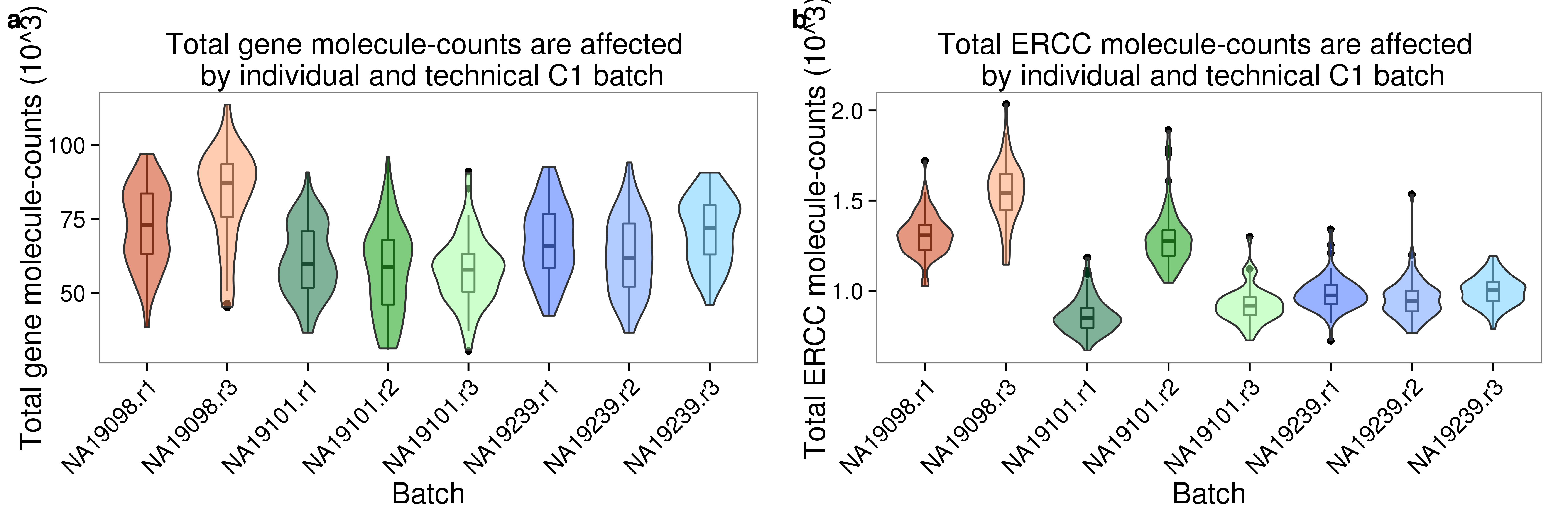
plot_grid(plot_conc_molecules_gene_individual +
            guides(shape = FALSE) + theme(legend.position = "bottom"),
          plot_gene_mol_ercc_mol +
            guides(shape = FALSE) + theme(legend.position = "bottom"),
          labels = letters[3:4])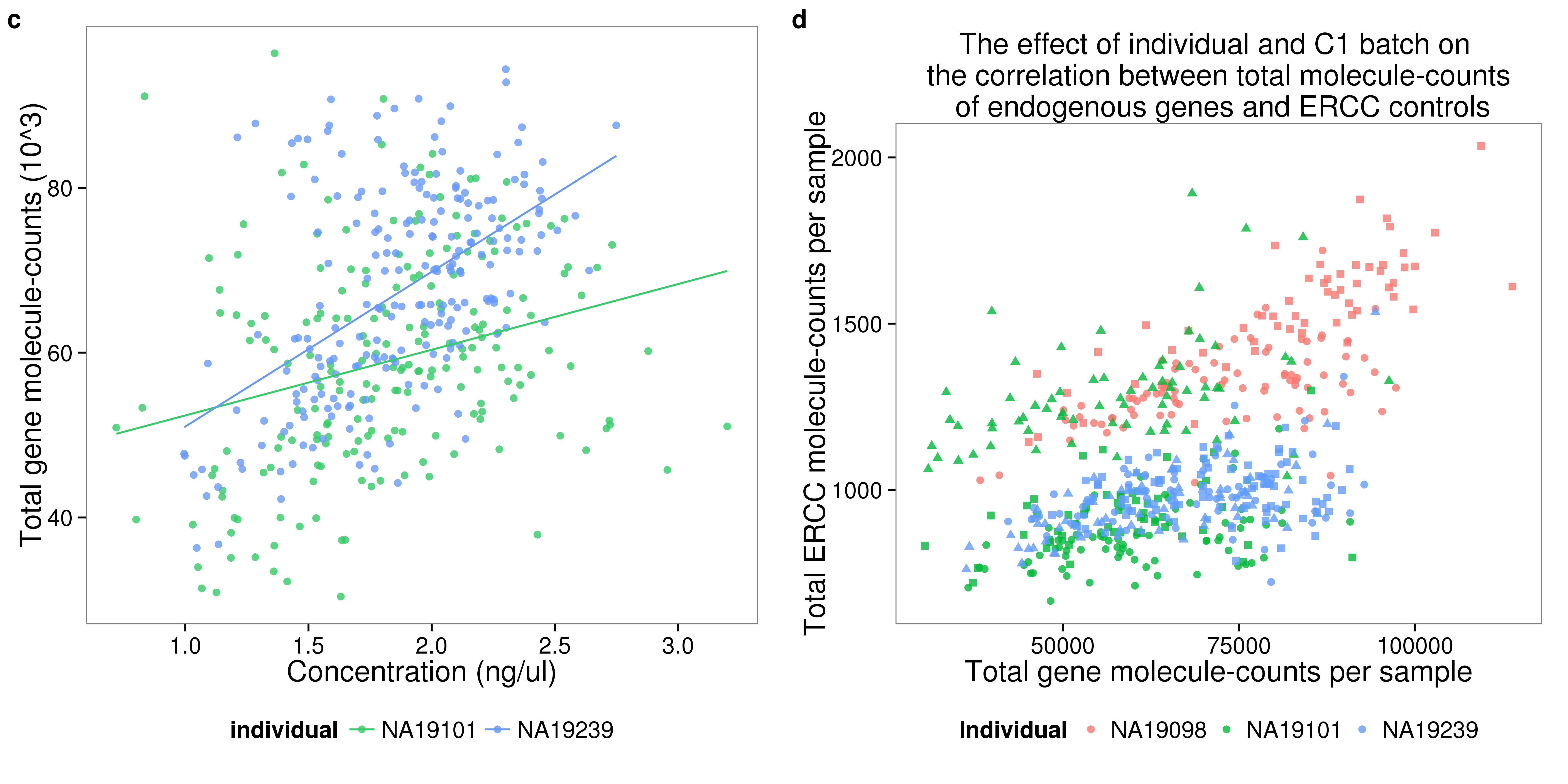
plot_grid(plot_total_molecules_ercc + theme(legend.position = "none"),
          plot_gene_mol_ercc_mol +
          theme(legend.position = "bottom"),
          labels = letters[1:2])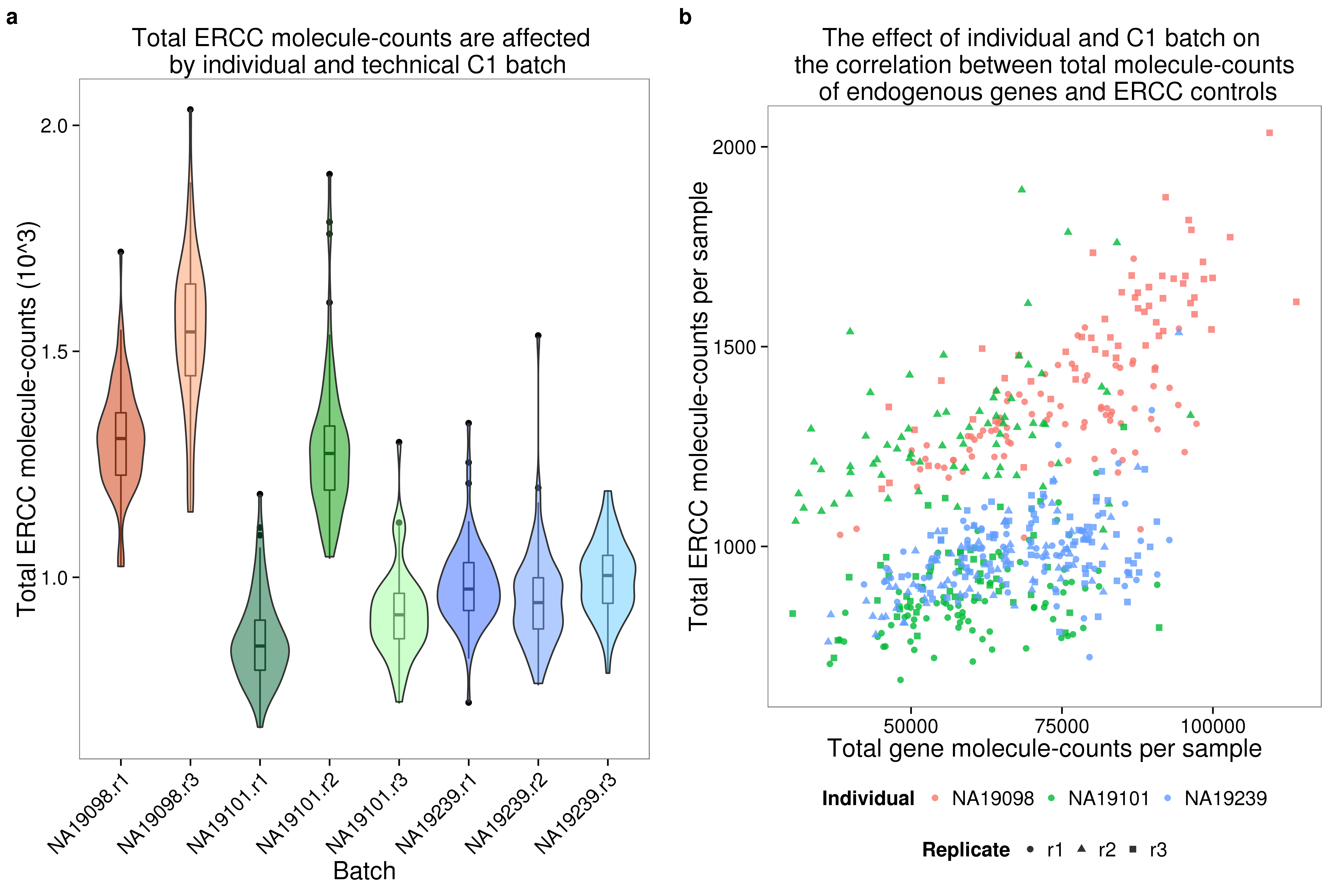
Expression profile
## pca of endogenous genes
pca_molecules_profile_ENSG <- run_pca(molecules[!ercc_index, ])
pca_molecules_ENSG_plot <- plot_pca(pca_molecules_profile_ENSG$PCs,
         explained = pca_molecules_profile_ENSG$explained,
         metadata = anno_single, color = "individual",
         shape = "replicate", alpha = 0.5, size = 2.2) +
  labs(title = "Endogenous gene expression profile")


## pca of ERCC spike-ins
pca_molecules_profile_ERCC <- run_pca(molecules[ercc_index, ])
pca_molecules_ERCC_plot <- plot_pca(pca_molecules_profile_ERCC$PCs,
         explained = pca_molecules_profile_ERCC$explained,
         metadata = anno_single, color = "individual",
         shape = "replicate", alpha = 0.5, size = 2.2) +
  labs(title = "ERCC spike-in expression profile")

## make plots
plot_grid(pca_molecules_ENSG_plot + theme(legend.position = "none"),
          pca_molecules_ERCC_plot + theme(legend.position = "none"),
          labels = LETTERS[1:2])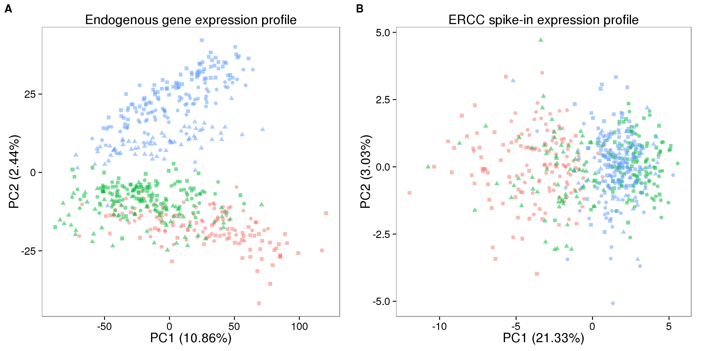
Session information
sessionInfo()R version 3.2.0 (2015-04-16)
Platform: x86_64-unknown-linux-gnu (64-bit)
locale:
[1] LC_CTYPE=en_US.UTF-8 LC_NUMERIC=C
[3] LC_TIME=en_US.UTF-8 LC_COLLATE=en_US.UTF-8
[5] LC_MONETARY=en_US.UTF-8 LC_MESSAGES=en_US.UTF-8
[7] LC_PAPER=en_US.UTF-8 LC_NAME=C
[9] LC_ADDRESS=C LC_TELEPHONE=C
[11] LC_MEASUREMENT=en_US.UTF-8 LC_IDENTIFICATION=C
attached base packages:
[1] stats graphics grDevices utils datasets methods base
other attached packages:
[1] testit_0.4 cowplot_0.3.1 ggplot2_1.0.1 lmtest_0.9-34 zoo_1.7-12
[6] edgeR_3.10.2 limma_3.24.9 tidyr_0.2.0 dplyr_0.4.2 knitr_1.10.5
loaded via a namespace (and not attached):
[1] Rcpp_0.12.4 magrittr_1.5 MASS_7.3-40 munsell_0.4.3
[5] colorspace_1.2-6 lattice_0.20-31 R6_2.1.1 plyr_1.8.3
[9] stringr_1.0.0 httr_0.6.1 tools_3.2.0 parallel_3.2.0
[13] grid_3.2.0 gtable_0.1.2 DBI_0.3.1 htmltools_0.2.6
[17] lazyeval_0.1.10 yaml_2.1.13 assertthat_0.1 digest_0.6.8
[21] reshape2_1.4.1 formatR_1.2 bitops_1.0-6 RCurl_1.95-4.6
[25] evaluate_0.7 rmarkdown_0.6.1 labeling_0.3 stringi_1.0-1
[29] scales_0.4.0 proto_0.3-10