Intermediate programming with R
Instructor’s Guide
library("dplyr")
library("ggplot2")
library("testit")
This page contains the solutions to the exercises. Since most of the exercises use counts-raw.txt.gz, it is loaded here at the beginning. Also, many use research, the subset of the data that only includes research articles.
counts_raw <- read.delim("data/counts-raw.txt.gz")
research <- filter(counts_raw, articleType == "Research Article")
01 Setting up a project
Create a README file
It is a convention to have a file named README in a project directory to explain what it contains (both for others and your future self). Use nano to create a README file. Include the date and explain that this directory was created for a Software Carpentry workshop.
Looking for an answer something like the following:
nano README
cat REAMDME
This directory contains the files created during the Software Carpentry workshop
at X University on YYYY-MM-DD.02 Inspecting a file
Q: What could be the reason for the discrepancy in the number of articles in our saved file?
A: The first command searches only in column 11. The second looks for matches in any of the columns. Thus the second command returns more lines because these strings are also present in some other columns.
Largest number of Wikipedia cites
What is the largest number of Wikipedia cites that an article in this data set has received? Hint: The counts of Wikipedia cites are in column 28.
gunzip -c counts-raw.txt.gz | cut -f28 | sort -n | tail -n 117Alternatively:
gunzip -c counts-raw.txt.gz | cut -f28 | sort -nr | head -n 117Find articles in your field
Choose two PLOS subject tags to search for and save these articles to a new file. How many articles are there?
There are lots of possible subject tags to choose from:
gunzip -c counts-raw.txt.gz | cut -f11 | sort | uniq | wc -l6717As an example:
gunzip -c counts-raw.txt.gz | cut -f11 | grep "Cardiovascular Disorders" | grep "Nephrology" | wc -l1403 Using RStudio
Opening and closing RStudio projects
Using the same drop down menu at the top right of RStudio, which you used to create the project, choose to “Close Project”. In the Console run getwd. It should display your home folder. Furthermore, your home folder should be displayed in the Files pane. Now open the altmetrics project using the same menu and run getwd again. The working directory should have changed to thealtmetrics directory, and the Files pane should display its contents.
If the RStudio Project was setup correctly, this should be straightforward.
04 Importing and inspecting data
Citations versus weeks since publication
Create a scatter plot where the x-axis is the number of weeks since publication and the y-axis is the log of the 2011 citations (use wosCountThru2011). Don’t forget to add a pseudocount of 1.
plot(counts_raw$daysSincePublished / 7,
     log(counts_raw$wosCountThru2011 + 1))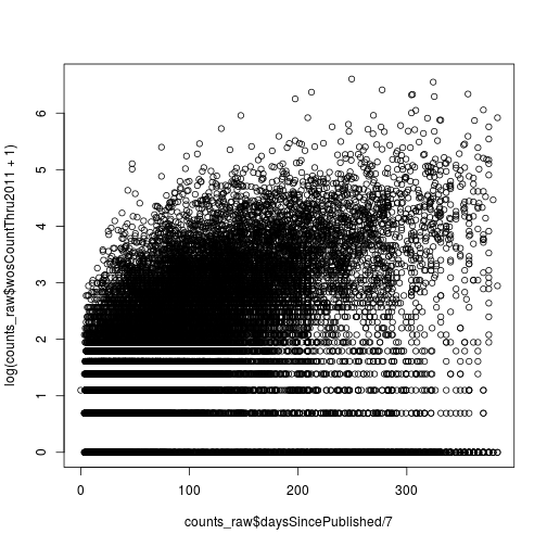
05 Conditional statments
Filtering articles
How many articles with the subject tag (plosSubjectTags) “Evolutionary Biology” were published in either PLOS One (“pone”), PLOS Biology (“pbio”), or PLOS Medicine (“pmed”)?
dim(counts_raw[grepl("Evolutionary Biology", counts_raw$plosSubjectTags) &
                 counts_raw$journal %in% c("pone", "pbio", "pmed"), ])
[1] 2080 32
06 Loops
Using apply
Using apply and sd, calculate the standard deviation of each row of counts_sub.
Using apply and max, calculate the maximum of each column of counts_sub.
counts_sub <- counts_raw[, c("wosCountThru2011", "backtweetsCount",
                             "plosCommentCount")]
sum_stat_sd <- apply(counts_sub, 1, sd)
summary(sum_stat_sd)
Min. 1st Qu. Median Mean 3rd Qu. Max.
0.000 1.155 3.464 7.832 8.563 425.500
apply(counts_sub, 2, max)wosCountThru2011 backtweetsCount plosCommentCount
737 363 49
07 Functions
Write your own function
Write your own function to calculate the mean called my_mean. It should take one input argument, x, which is a numeric vector. Compare your results with the results from R’s function mean. Do you receive the same answer?
my_mean <- function(x) {
  result <- sum(x) / length(x)
  return(result)
}
my_mean(1:10)
[1] 5.5
mean(1:10)[1] 5.5
11 R Markdown Output Options
Update analysis file
You need to share your initial results with your collaborators, but after showing your report to your boss, they had a few suggestions.
- In your final report, your collaborators should see your histogram of authors per paper, but not the code that produced the plot.
- The figure is hard to see as is, resize it to 8x8 inches
- Your collaborators are very interested in how popular articles are on Facebook. Add another histogram plotting the number of facebook shares per article (
facebookShareCount), ensuring there are respectible titles and axis labels. Also, just like the previous figure, make sure there is a legend and that the code to generate the figure does not appear in the final report. - Additionally under the new figure, your collaborators should see a sentence that says “The average number of Facebook shares per paper in the data set is X”, where X is the mean number of Facebook shares per paper, as evaluated by inline code.
- Use chunk option
echo=FALSE. - Use chunk options
fig.width=8, fig.height=8.
hist(counts_raw$facebookShareCount, xlab = "Number of shares on Facebook",
ylab = "Number of articles", main = "Distributin of Facebook Shares")- Use the inline code:
`r mean(counts_raw$facebookShareCount)`12 Subsetting with dplyr
How much did altmetrics numbers change by 2009?
How many articles were published in 2009 (year)? How many of these had at least one Tweet (backtweetsCount) or Facebook comment (facebookCommentCount)? How many were in at least one Mendeley library (mendeleyReadersCount)?
research_2009 <- filter(research, year == 2009)
nrow(research_2009)
[1] 6036
research_2009_fb_tweet <- filter(research, year == 2009,
                                 facebookCommentCount > 0 |
                                 backtweetsCount > 0)
nrow(research_2009_fb_tweet)
[1] 830
research_2009_mendeley <- filter(research, year == 2009,
                                 mendeleyReadersCount > 0)
nrow(research_2009_mendeley)
[1] 5078
What are people reading but not citing?
One potential use of altmetrics data is recognizing articles that are widely read among the scientific community but are not cited as highly as similarly influential papers. Compile a data set named low_cite that contains the journal, title, and year of each research article that meets the following criteria:
- Published in 2008 or prior (
year) - Has more than 1,000 pdf downloads (
pdfDownloadsCount) - Is contained in more than 15 Mendeley libraries (
mendeleyReadersCount) - Has fewer than 10 citations as of 2011 (
wosCountThru2011)
How many articles did you find?
summary(research$pdfDownloadsCount) Min. 1st Qu. Median Mean 3rd Qu. Max.
0.0 152.0 261.0 432.5 481.0 35720.0
summary(research$mendeleyReadersCount) Min. 1st Qu. Median Mean 3rd Qu. Max.
0.000 1.000 2.000 4.128 5.000 171.000
summary(research$wosCountThru2011) Min. 1st Qu. Median Mean 3rd Qu. Max.
0.00 2.00 7.00 14.54 16.00 737.00
low_cite <- filter(research, pdfDownloadsCount > 1000,
                   mendeleyReadersCount > 15,
                   year < 2009, wosCountThru2011 < 10)
low_cite <- select(low_cite, journal, title, year)
nrow(low_cite)
[1] 25
13 Chaining commands with dplyr
Titles of most cited articles
Using a chain of pipes, output the titles of the three research articles with the largest 2011 citation count (wosCountThru2011).
Lots of authors
Using a chain of pipes, output the author count (authorsCount), title, journal, and subject tags (plosSubjectTags) of the three research articles with the largest number of authors.
14 Summarizing with dplyr
Summarizing the number of tweets per journal
Create a new data frame, tweets_per_journal, that for each journal contains the total number of articles, the mean number of tweets (backtweetsCount) received by articles in that journal, and the standard error of the mean (SEM) of the number of tweets. The SEM is the standard deviation divided by the square root of the sample size (i.e. the number of articles).
tweets_per_journal <- research %>%
  group_by(journal) %>%
  summarize(num = n(),
            mean = mean(backtweetsCount),
            sem = sd(backtweetsCount) / sqrt(num))
tweets_per_journal
Source: local data frame [7 x 4]
journal num mean sem
<fctr> <int> <dbl> <dbl>
1 pbio 1325 0.05811321 0.020153395
2 pcbi 1351 0.12657291 0.052177184
3 pgen 1619 0.06547251 0.020408525
4 pmed 643 0.31104199 0.187868371
5 pntd 621 0.02576490 0.009057697
6 pone 14078 0.49303878 0.034484187
7 ppat 1459 0.02604524 0.008807428
15 Mapping data to plot aesthetics
Citations versus days since publication
Create a scatter plot with daysSincePublished mapped to the x-axis and wosCountThru2011 mapped to the y-axis. Include a loess fit of the data. Set the transparency level (alpha) of the points to 0.5 and color the points according to the journal where the article was published. Make the loess curve red.
p <- ggplot(research, aes(x = daysSincePublished,
                          y = wosCountThru2011)) +
  geom_point(aes(color = journal), alpha = 0.5) +
  geom_smooth(color = "red")
p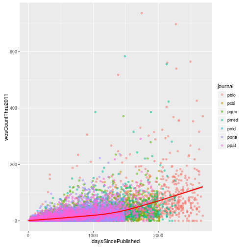
16 Controlling the plot scales
Modifying the scales
Update the plot to use a square root transformation instead of log10. Also color the points using the ColorBrewer palette “Accent”.
p <- ggplot(research, aes(x = pdfDownloadsCount,
                          y = wosCountThru2011)) +
  geom_point(aes(color = journal)) +
  geom_smooth() +
  scale_x_sqrt() +
  scale_y_sqrt() +
  scale_color_brewer(palette = "Accent")
p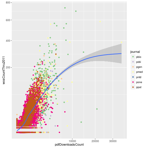
17 Creating subplots with facets
Using facets
Add another variable to research called evolution, which is a logical vector indicating if the article has the PLOS subject tag “Evolutionary Biology”. Use facet_grid to create subplots based on the variables evolution and immuno.
# From earlier in the lesson
research <- mutate(research, immuno = grepl("Immunology", plosSubjectTags))
# Solution:
research <- mutate(research,
                   evolution = grepl("Evolutionary Biology",
                                     plosSubjectTags))
p <- ggplot(research, aes(x = log10(pdfDownloadsCount + 1),
                          y = log10(wosCountThru2011 + 1))) +
  geom_point(aes(color = journal)) +
  geom_smooth() +
  scale_x_continuous(breaks = c(1, 3), labels = c(10, 1000)) +
  scale_y_continuous(breaks = c(1, 3), labels = c(10, 1000)) +
  facet_grid(evolution~immuno)
p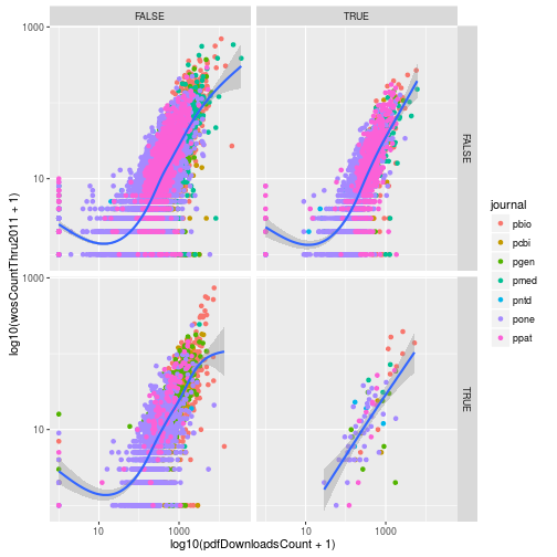
18 Creating different plots with geoms
Mean number of tweets per journal per year
Modify the dplyr code above to calculate the mean, SEM, and sample size of the number of article tweets per journal and per year. Use facet_wrap to make a separate subplot per year.
tweets_per_journal_year <- research %>%
  group_by(journal, year) %>%
  summarize(num = n(),
            mean = mean(backtweetsCount),
            sem = sd(backtweetsCount) / sqrt(num))
tweets_per_journal_year
Source: local data frame [42 x 5]
Groups: journal [?]
journal year num mean sem
<fctr> <int> <int> <dbl> <dbl>
1 pbio 2003 33 0.000000000 0.000000000
2 pbio 2004 174 0.000000000 0.000000000
3 pbio 2005 176 0.011363636 0.008012313
4 pbio 2006 184 0.010869565 0.007664915
5 pbio 2007 203 0.004926108 0.004926108
6 pbio 2008 197 0.030456853 0.018916893
7 pbio 2009 181 0.005524862 0.005524862
8 pbio 2010 177 0.367231638 0.146996329
9 pcbi 2005 55 0.000000000 0.000000000
10 pcbi 2006 136 0.000000000 0.000000000
.. ... ... ... ... ...
ggplot(tweets_per_journal_year, aes(x = journal, y = mean)) +
  geom_bar(stat = "identity") +
  geom_errorbar(aes(ymin = mean - sem, ymax = mean + sem), width = 0.1) +
  geom_text(aes(label = num), hjust = 0, vjust = 0) +
  facet_wrap(~year)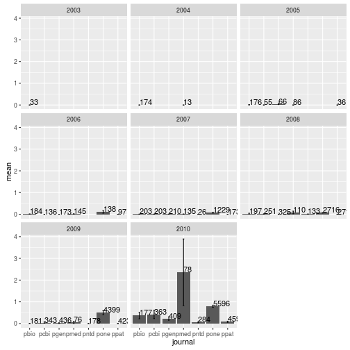
Visualizing a single distribution
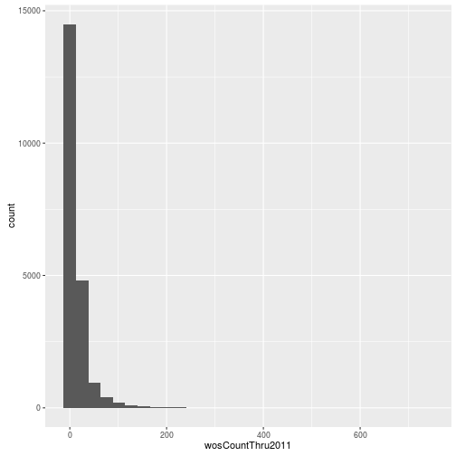
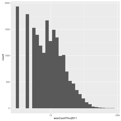
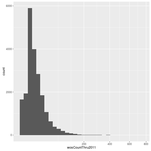
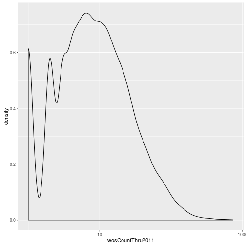
The geoms geom_histogram and geom_density can be used to create histograms and density plots, respectively. Using these geoms, visualize the distribution of 2011 citations (wosCountThru2011). Compare the raw distribution to log10 and square root transformations.
p <- ggplot(research, aes(x = wosCountThru2011))
p + geom_histogram()
`stat_bin()` using `bins = 30`. Pick better value with `binwidth`.
p + geom_histogram() + scale_x_log10() `stat_bin()` using `bins = 30`. Pick better value with `binwidth`.
Warning: Removed 1654 rows containing non-finite values (stat_bin).
p + geom_histogram() + scale_x_sqrt()`stat_bin()` using `bins = 30`. Pick better value with `binwidth`.
p + geom_density()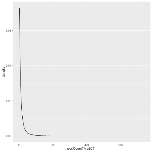
p + geom_density() + scale_x_log10() Warning: Removed 1654 rows containing non-finite values (stat_density).
p + geom_density() + scale_x_sqrt()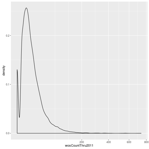
20 Debugging with debug
Limit to a subset of levels
What if we were only interested in the mean of the number of tweets in the journals PLOS Biology (pbio) and PLOS One (pone)? We could subset to only pass values for these journals to the function mean_metric_per_var.
mean_metric_per_var(counts_raw$backtweetsCount[counts_raw$journal %in% c("pbio", "pone")],
                   counts_raw$journal[counts_raw$journal %in% c("pbio", "pone")])
pbio pcbi pgen pmed pntd pone ppat
0.0555770 NaN NaN NaN NaN 0.4942194 NaN
Unfortunately this still gives us results for the other journals. And their result is NaN, a special value indiciating “Not a Number”.
Use debug to isolate and diagnose the problem.
As an added challenge, can you fix the bug?
# Use droplevels
mean_metric_per_var <- function(metric, variable) {
  if (!is.factor(variable)) {
    variable <- as.factor(variable)
  }
  variable <- droplevels(variable)
  result <- numeric(length = length(levels(variable)))
  names(result) <- levels(variable)
  for (v in levels(variable)) {
    result[v] <- mean(metric[variable == v])
  }
  return(result)
}
mean_metric_per_var(counts_raw$backtweetsCount[counts_raw$journal %in% c("pbio", "pone")],
                   counts_raw$journal[counts_raw$journal %in% c("pbio", "pone")])
pbio pone
0.0555770 0.4942194
23 Defensive programming with stopifnot
Practice defensive programming
Use defensive programming techniques to make the function calc_sum_stat more robust.
calc_sum_stat <- function(df, cols) {
  df_sub <- df[, cols, drop = FALSE]
  sum_stat <- apply(df_sub, 1, mean)
  return(sum_stat)
}
Some specific ideas:
- Assert that the input
dfis not empty (hint: usedim) - Assert that
colsis a character vector - Assert that the columns listed in
colsare indf(hint: use%in%andcolnames) - Assert that
df_subis a data frame (hint: useis.data.frame) - Assert that
sum_statis notNA - Issue a warning if
colsonly contains one column (since taking the mean of one column isn’t very useful, the user may have made a mistake)
After you add your assertion statements, test out the following inputs to calc_sum_stat. Do your assertion statements catch these errors? Should we update the function based on some of these results?
# Empty data frame
sum_stat <- calc_sum_stat(data.frame(), c("wosCountThru2010", "f1000Factor"))
# Non-character cols
sum_stat <- calc_sum_stat(counts_raw, 1:3)
# Bad column names
sum_stat <- calc_sum_stat(counts_raw, c("a", "b"))
# Issue warning since only one column
sum_stat <- calc_sum_stat(counts_raw, "mendeleyReadersCount")
# NA output
sum_stat <- calc_sum_stat(counts_raw, c("wosCountThru2010", "facebookLikeCount"))
# Because of the `NA` result, use `na.rm = TRUE` with `mean`
calc_sum_stat <- function(df, cols) {
stopifnot(dim(df) > 0,
is.character(cols),
cols %in% colnames(df))
if (length(cols) == 1) {
warning("Only one column specified. Calculating the mean will not change anything.")
}
df_sub <- df[, cols, drop = FALSE]
stopifnot(is.data.frame(df_sub))
sum_stat <- apply(df_sub, 1, mean, na.rm = TRUE)
stopifnot(!is.na(sum_stat))
return(sum_stat)
}
# Proper
sum_stat <- calc_sum_stat(counts_raw, c("wosCountThru2010", "f1000Factor"))24 Testing with testit
Write some tests
Write unit tests for the function my_mean that you wrote in an earlier lesson. It should look something like this:
my_mean <- function(x) {
  result <- sum(x) / length(x)
  return(result)
}
The input x is a numeric vector, and the output is the mean of the vector of numbers. Some ideas to get started:
- Pass a vector where you know what the mean is, and assert that the result is correct.
- Add some assertion statments to check the input
x. Usehas_errorto test that the function throws an error when given bad input. - Issue a warning if the user passes a vector of length one. Test that the warning is properly issued using
has_warning. - Include an
NAin the vector where you know the result to see what happens. Do you need to modify the code to pass the test?
my_mean <- function(x) {
  assert("x is numeric", is.numeric(x))
  if (length(x) == 1) {
    warning("Input vector had only one element")
  }
  result <- sum(x, na.rm = TRUE) / length(x[!is.na(x)])
  return(result)
}

assert("Mean is calculated correctly",
       my_mean(1:3) == 2, my_mean(c(2, 4, 6)) == 4)
assert("Non-numeric input throws error",
       has_error(my_mean("hello")))
assertion failed: x is numeric
assert("Input vector with one element issues warning",
       has_warning(my_mean(5)))
assert("Mean is calculated correctly when given NAs",
       my_mean(c(2, 4, 6, NA)) == 4)