BASiCS - 40,000 iterations
2015-08-10
Last updated: 2015-11-11
Code version: 48d0a820ba6794f241a52faf89a214afeba506d9
We analyzed our single cell data with BASiCS developed by Vallejos et al., 2015. The results shown here are from a model fit with 40,000 iterations. This time we also modeled the unexplained technical noise with a separate parameter (theta) per batch.
BASiCS and its dependency, RcppArmadillo, were able to be installed on the cluster using a new version of gcc. Since this took a long time to run, it was submitted via the following:
echo "Rscript -e 'library(rmarkdown); render(\"basics.Rmd\")'" | \
  qsub -l h_vmem=32g -cwd -V -j y -o ~/log/ -N basics
library("BASiCS")
library("data.table")
source("functions.R")
library("ggplot2")
theme_set(theme_bw(base_size = 16))
library("tidyr")
library("edgeR")Loading required package: limmaInput
Below is the description of the data from the BASiCS vignette, interspersed with my code to load the data.
The input dataset for BASiCS must contain the following 3 elements:
Counts: a matrix of raw expression counts with dimensions q times n. First q0 rows must correspond to biological genes. Last q − q0 rows must correspond to technical spike-in genes.
Input annotation.
anno_filter <- read.table("../data/annotation-filter.txt", header = TRUE,
                          stringsAsFactors = FALSE)
Input molecule counts.
molecules_filter <- read.table("../data/molecules-filter.txt", header = TRUE,
                               stringsAsFactors = FALSE)
stopifnot(nrow(anno_filter) == ncol(molecules_filter),
          colnames(molecules_filter) == anno_filter$sample_id,
          anno_filter$well != "bulk")
Remove outlier batch NA19098.r2.
molecules_filter <- molecules_filter[, anno_filter$batch != "NA19098.r2"]
anno_filter <- anno_filter[anno_filter$batch != "NA19098.r2", ]
stopifnot(nrow(anno_filter) == ncol(molecules_filter),
          colnames(molecules_filter) == anno_filter$sample_id,
          anno_filter$well != "bulk")
Tech: a vector ofTRUE/FALSEelements with length q. IfTech[i] = FALSEthe geneiis biological; otherwise the gene is spike-in.
tech <- grepl("ERCC", rownames(molecules_filter))
SpikeInput: a vector of length q − q0 whose elements contain the input number of molecules for the spike-in genes (amount per cell).
spike <- read.table("../data/expected-ercc-molecules.txt", header = TRUE,
                    sep = "\t", stringsAsFactors = FALSE)
Only keep the spike-ins that were observed in at least one cell.
spike_input <- spike$ercc_molecules_well[spike$id %in% rownames(molecules_filter)]
names(spike_input) <- spike$id[spike$id %in% rownames(molecules_filter)]
spike_input <- spike_input[order(names(spike_input))]
stopifnot(sum(tech) == length(spike_input),
          rownames(molecules_filter)[tech] == names(spike_input))
34 of the ERCC spike-ins were observed in the single cell data.
These elements must be stored into an object of class
BASiCS_Data.
basics_data <- newBASiCS_Data(as.matrix(molecules_filter), tech, spike_input,
                              BatchInfo = anno_filter$batch)
An object of class BASiCS_Data
Dataset contains 10598 genes (10564 biological and 34 technical) and 568 cells.
Elements (slots): Counts, Tech, SpikeInput and BatchInfo.
The data contains 8 batches.
NOTICE: BASiCS requires a pre-filtered dataset
- You must remove poor quality cells before creating the BASiCS data object
- We recommend to pre-filter very lowly expressed transcripts before creating the object.
Inclusion criteria may vary for each data. For example, remove transcripts
- with very low total counts across of all samples
- that are only expressed in few cells
(by default genes expressed in only 1 cell are not accepted)
- with very low total counts across the samples where the transcript is expressed
BASiCS_Filter can be used for this purpose Fit the model
store_dir <- "../data"
run_name <- "batch-clean"
if (file.exists(paste0(store_dir, "/chain_phi_", run_name, ".txt"))) {
  chain_mu = as.matrix(fread(paste0(store_dir, "/chain_mu_", run_name, ".txt")))
  chain_delta = as.matrix(fread(paste0(store_dir, "/chain_delta_", run_name, ".txt")))
  chain_phi = as.matrix(fread(paste0(store_dir, "/chain_phi_", run_name, ".txt")))
  chain_s = as.matrix(fread(paste0(store_dir, "/chain_s_", run_name, ".txt")))
  chain_nu = as.matrix(fread(paste0(store_dir, "/chain_nu_", run_name, ".txt")))
  chain_theta = as.matrix(fread(paste0(store_dir, "/chain_theta_", run_name, ".txt")))

  mcmc_output <- newBASiCS_Chain(mu = chain_mu, delta = chain_delta,
                                 phi = chain_phi, s = chain_s,
                                 nu = chain_nu, theta = chain_theta)

  time_total <- readRDS(paste0(store_dir, "/time_total_", run_name, ".rds"))
} else {
  time_start <- Sys.time()
  mcmc_output <- BASiCS_MCMC(basics_data, N = 40000, Thin = 10, Burn = 20000,
                             PrintProgress = TRUE, StoreChains = TRUE,
                             StoreDir = store_dir, RunName = run_name)
  time_end <- Sys.time()
  time_total <- difftime(time_end, time_start, units = "hours")
  saveRDS(time_total, paste0(store_dir, "/time_total_", run_name, ".rds"))
}
Read 0.0% of 2000 rows
Read 2000 rows and 10598 (of 10598) columns from 0.333 GB file in 00:00:08

Read 0.0% of 2000 rows
Read 2000 rows and 10564 (of 10564) columns from 0.351 GB file in 00:00:09
An object of class BASiCS_Chain
 2000 MCMC samples.
 Dataset contains 10598 genes (10564 biological and 34 technical) and 568 cells (8 batches).
 Elements (slots): mu, delta, phi, s, nu and theta.
Fitting the model took 79.66 hours.
Summarize the results.
mcmc_summary <- Summary(mcmc_output)Batch information
The unexplained technical noise is similar across batches.
colnames(mcmc_output@theta) <- unique(anno_filter$batch)
theta_long <- gather(as.data.frame(mcmc_output@theta), key = "batch",
                     value = "theta")
ggplot(theta_long, aes(x = batch, y = theta)) +
  geom_boxplot() +
  theme(axis.text.x = element_text(angle = 90)) +
  labs(title = "Modeling of separate technical effects per batch")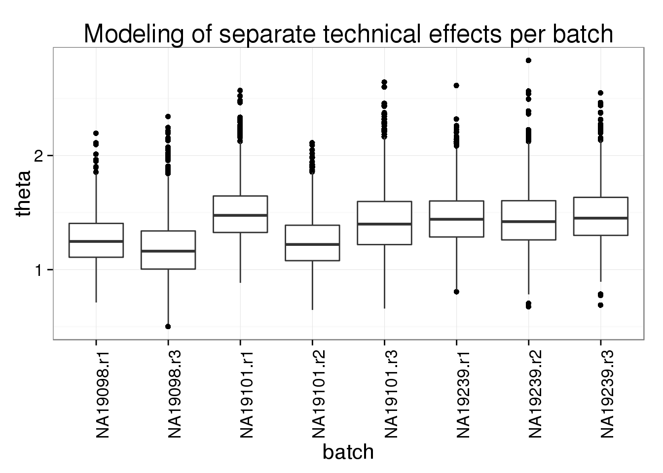
Cell-specific normalizing constants
BASiCS models two cell-specific parameters. Phi models the differences in gene molecules. S models the differences in ERCC molecules.
plot(mcmc_summary, Param = "phi")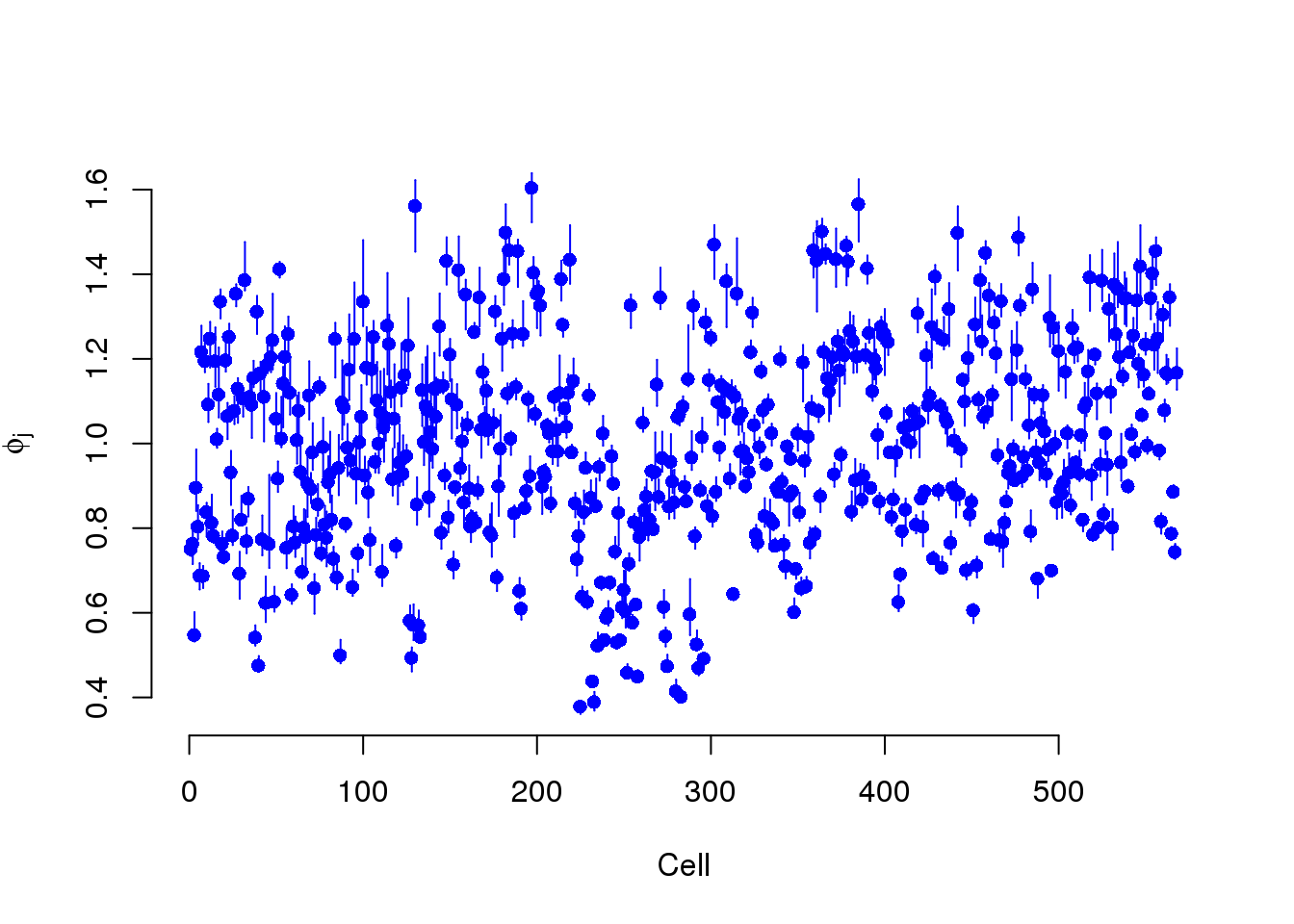
plot(mcmc_summary, Param = "s")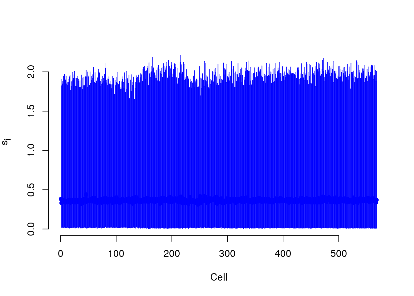
phi <- displaySummaryBASiCS(mcmc_summary, Param = "phi")
s <- displaySummaryBASiCS(mcmc_summary, Param = "s")
parameters <- cbind(phi, s, anno_filter)
parameters$gene_count <- colSums(counts(basics_data, type = "biological"))
parameters$ercc_count <- colSums(counts(basics_data, type = "technical"))
Phi versus gene molecule count
phi_gene_count <- ggplot(parameters, aes(x = gene_count, y = Phi)) +
  geom_point() +
  geom_smooth(method = "lm") +
  labs(x = "Gene molecule count",
       title = paste0("Phi measures gene molecule count differences\nr = ",
                      round(cor(parameters$gene_count, parameters$Phi), 2)))
phi_gene_count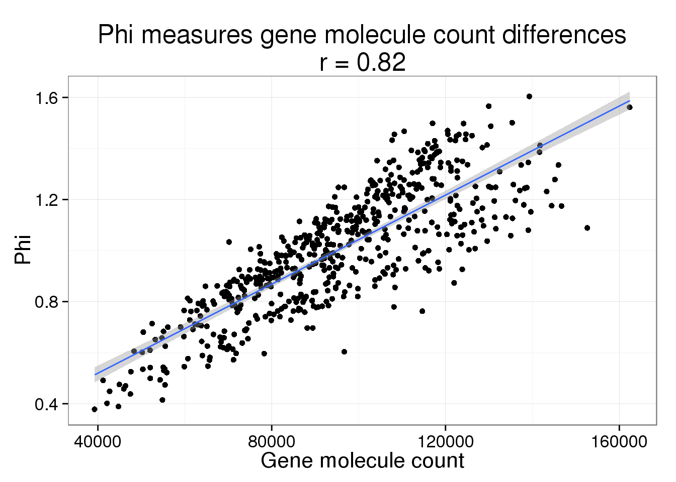
Phi versus ERCC molecule count
phi_ercc_count <- phi_gene_count %+% aes(x = ercc_count) +
  labs(x = "ERCC molecule count",
       title = paste0("Phi does not measure ERCC molecule count differences\nr = ",
                      round(cor(parameters$ercc_count, parameters$Phi), 2)))
phi_ercc_count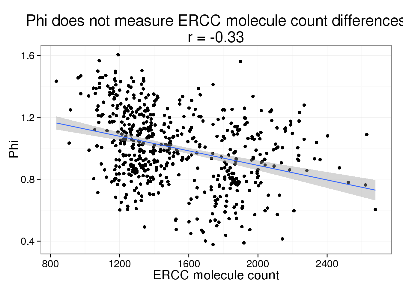
S versus ERCC molecule count
s_ercc_count <- phi_ercc_count %+% aes(y = S) +
  labs(y = "S",
       title = paste0("S measures ERCC molecule count differences\nr = ",
                      round(cor(parameters$ercc_count, parameters$S), 2)))
s_ercc_count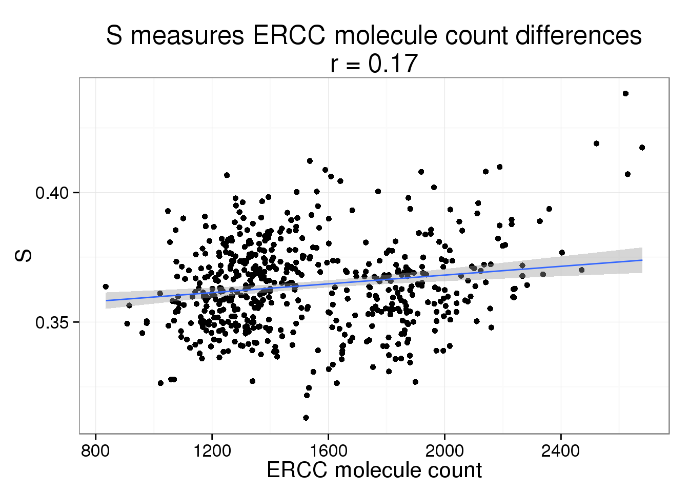
S versus gene molecule count
s_gene_count <- phi_gene_count %+% aes(y = S) +
  labs(y = "S",
       title = paste0("S does not measure gene molecule count differences\nr = ",
                      round(cor(parameters$gene_count, parameters$S), 2)))
s_gene_count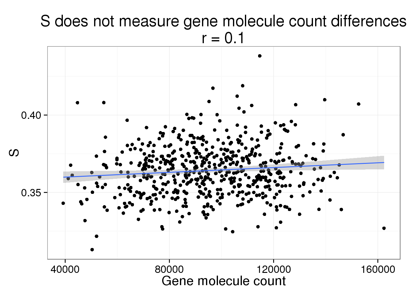
Phi versus S
phi_s <- ggplot(parameters, aes(x = S, y = Phi)) +
  geom_point() +
  geom_smooth(method = "lm") +
  labs(       title = paste0("Phi versus S\nr = ",
                      round(cor(parameters$S, parameters$Phi), 2)))
phi_s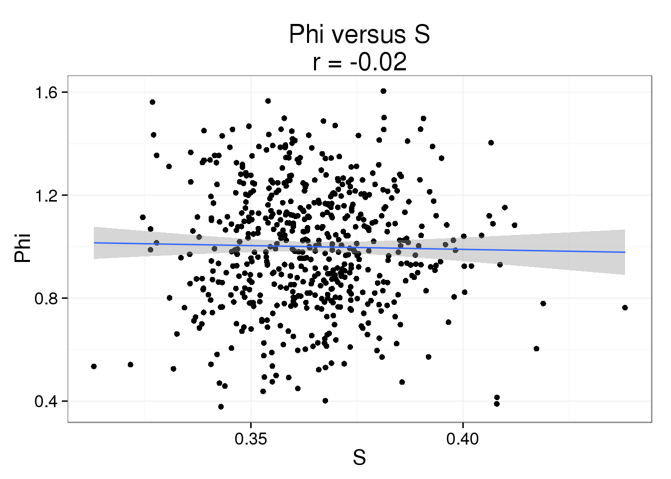
Denoised data
Remove technical noise (i.e. normalize using the ERCC spike-ins). This takes a long time!
denoised = BASiCS_DenoisedCounts(Data = basics_data, Chain = mcmc_output)
write.table(denoised, "../data/basics-denoised.txt", quote = FALSE,
            sep = "\t", col.names = NA)
denoised_rates = BASiCS_DenoisedRates(Data = basics_data, Chain = mcmc_output)
[1] "This calculation requires a loop across the 2000 MCMC iterations"
[1] "You might need to be patient ... "write.table(denoised_rates, "../data/basics-denoised-rates.txt", quote = FALSE,
sep = "\t", col.names = NA)PCA - BASiCS Denoised
Both the raw and the cpm versions of the BASiCS denoised data appear similar to the result with the non-normalized cpm data. This does not change substantially when increasing the iterations from a few thousands to a few tens of thousands.
pca_basics <- run_pca(denoised)
plot_pca(pca_basics$PCs, explained = pca_basics$explained,
         metadata = anno_filter, color = "individual",
         shape = "replicate")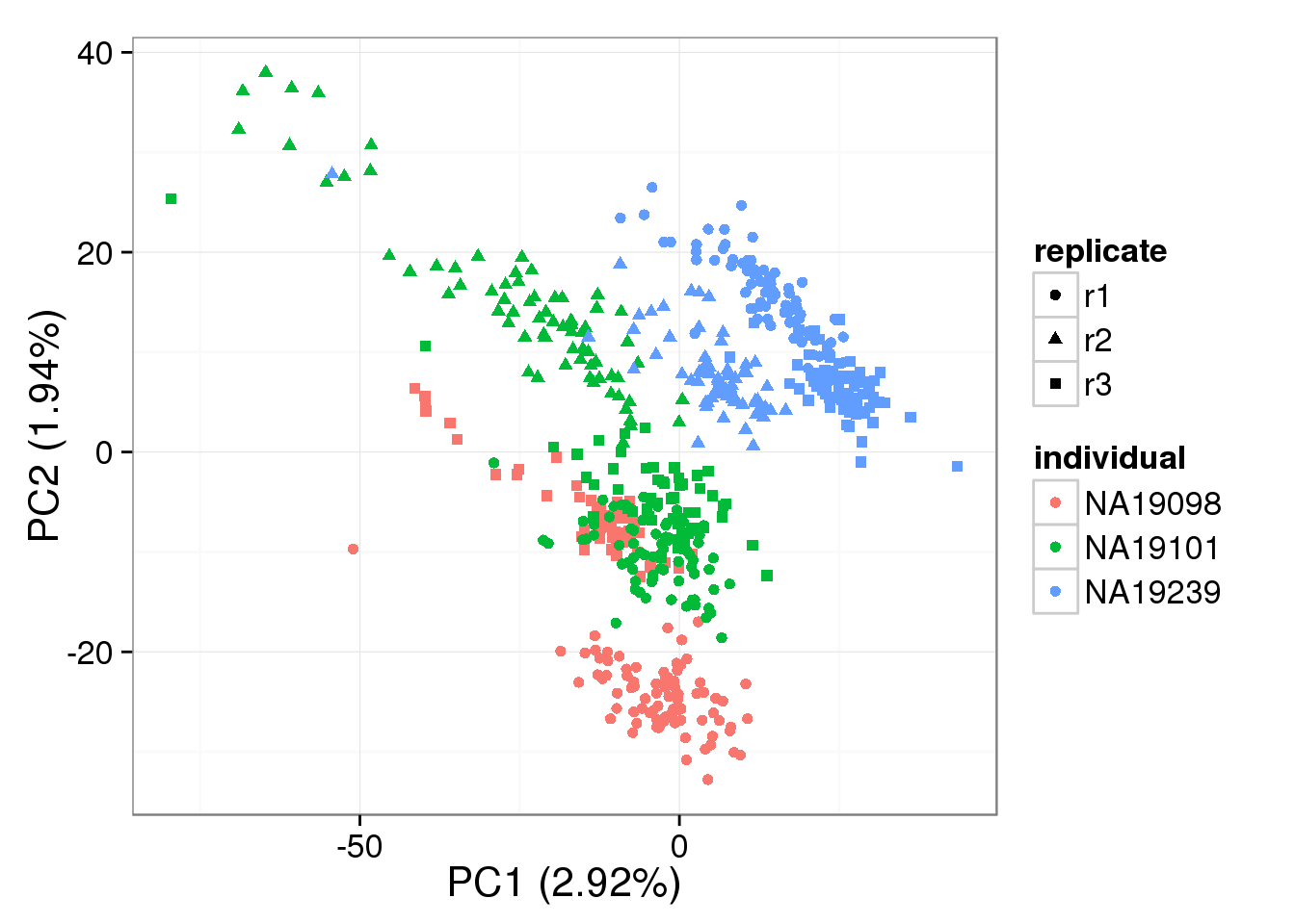
PCA - BASiCS Denoised cpm
denoised_cpm <- cpm(denoised, log = TRUE,
                    lib.size = colSums(denoised) *
                               calcNormFactors(denoised, method = "TMM"))
pca_basics_cpm <- run_pca(denoised_cpm)
plot_pca(pca_basics_cpm$PCs, explained = pca_basics_cpm$explained,
         metadata = anno_filter, color = "individual",
         shape = "replicate")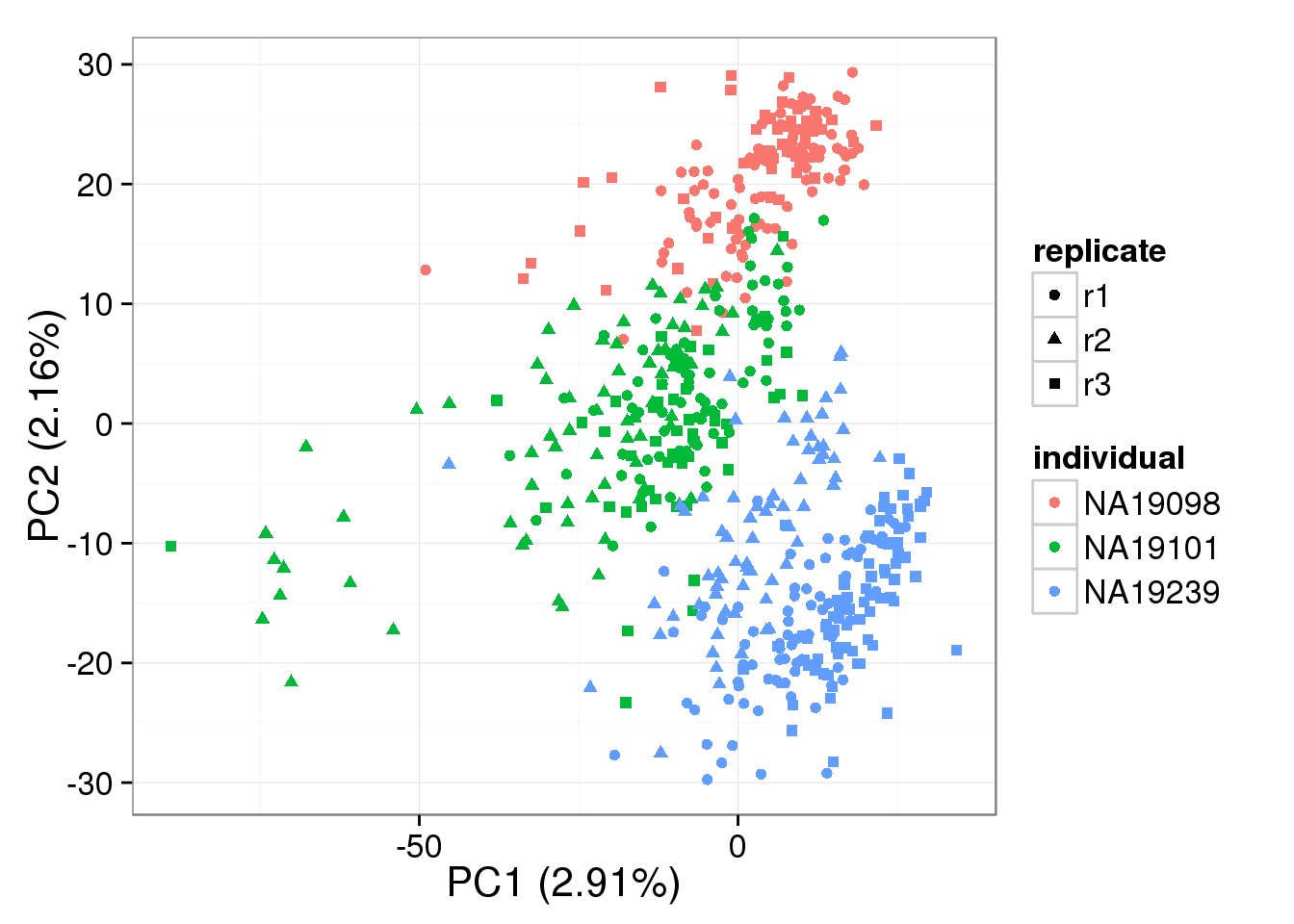
PCA - non-normalized
pca_non <- run_pca(counts(basics_data))
plot_pca(pca_non$PCs, explained = pca_non$explained,
         metadata = anno_filter, color = "individual",
         shape = "replicate")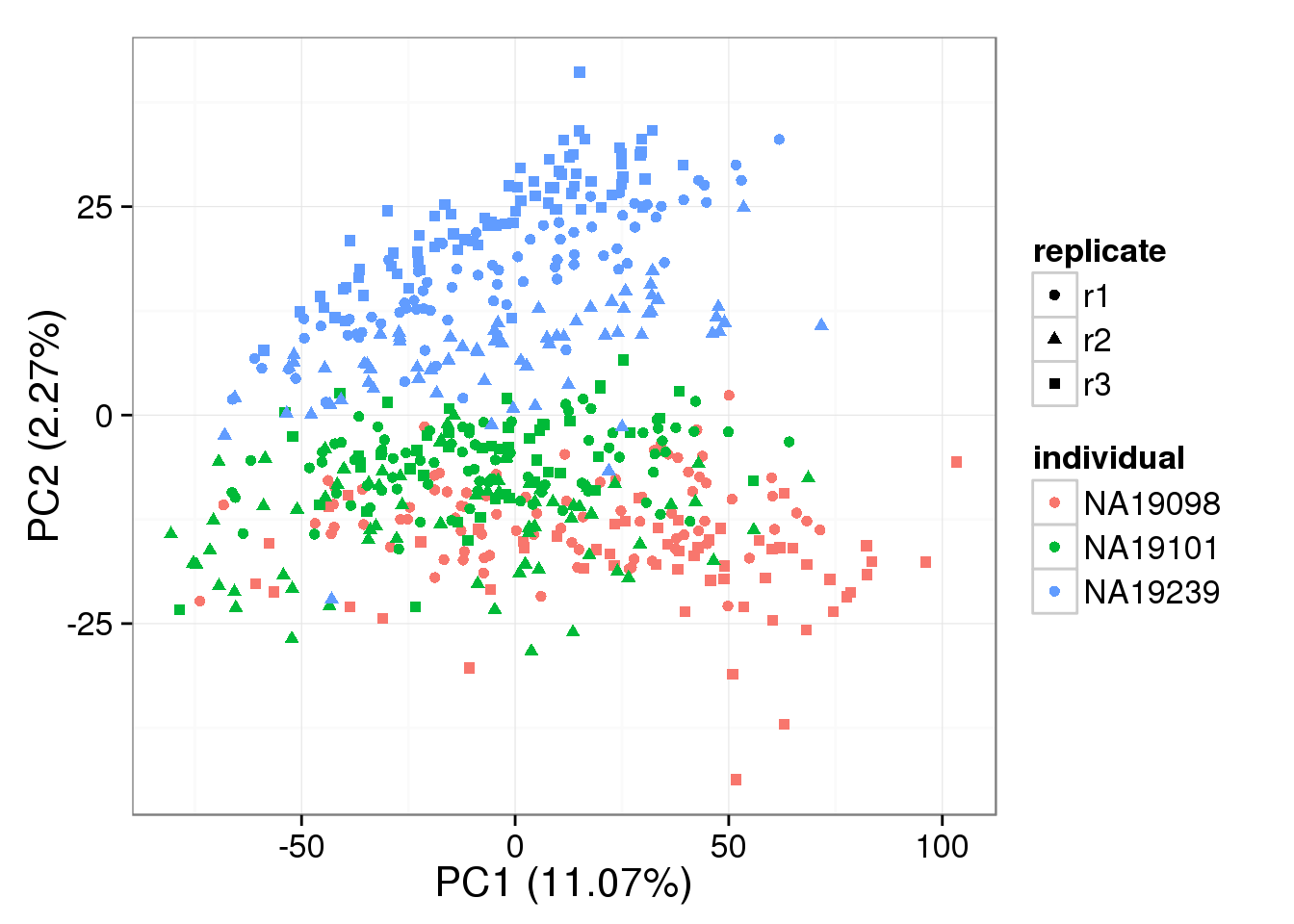
PCA - non-normalized cpm
non_cpm <- cpm(counts(basics_data), log = TRUE,
               lib.size = colSums(counts(basics_data)) *
                          calcNormFactors(counts(basics_data), method = "TMM"))
pca_non_cpm <- run_pca(non_cpm)
plot_pca(pca_non_cpm$PCs, explained = pca_non_cpm$explained,
         metadata = anno_filter, color = "individual",
         shape = "replicate")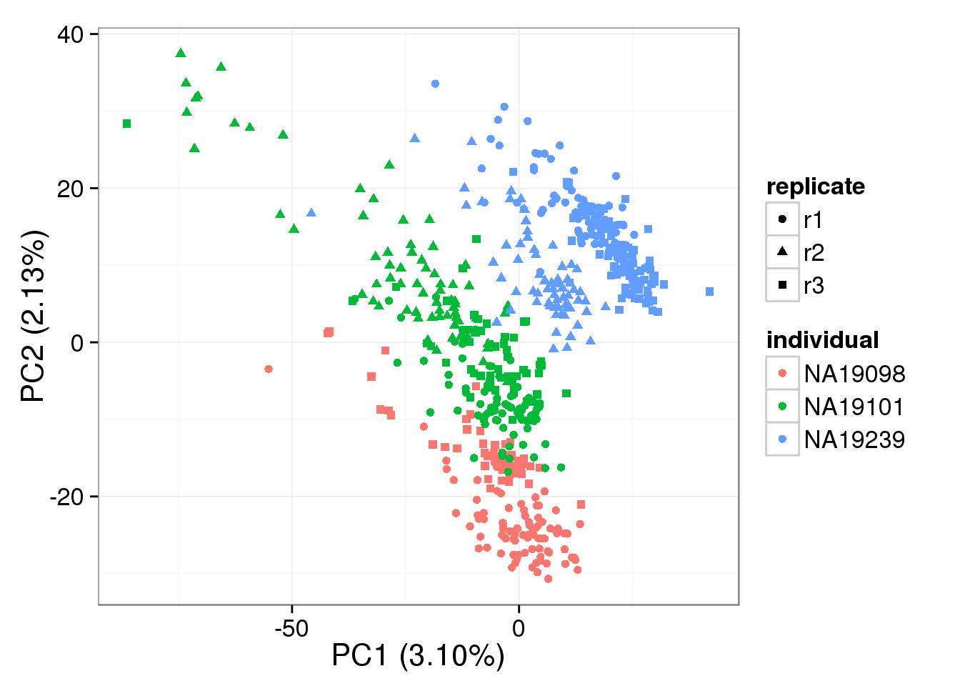
Session information
sessionInfo()R version 3.2.0 (2015-04-16)
Platform: x86_64-unknown-linux-gnu (64-bit)
locale:
[1] LC_CTYPE=en_US.UTF-8 LC_NUMERIC=C
[3] LC_TIME=en_US.UTF-8 LC_COLLATE=en_US.UTF-8
[5] LC_MONETARY=en_US.UTF-8 LC_MESSAGES=en_US.UTF-8
[7] LC_PAPER=en_US.UTF-8 LC_NAME=C
[9] LC_ADDRESS=C LC_TELEPHONE=C
[11] LC_MEASUREMENT=en_US.UTF-8 LC_IDENTIFICATION=C
attached base packages:
[1] stats graphics grDevices utils datasets methods base
other attached packages:
[1] testit_0.4 edgeR_3.10.2 limma_3.24.9 tidyr_0.2.0
[5] ggplot2_1.0.1 data.table_1.9.4 BASiCS_0.3.0 knitr_1.10.5
loaded via a namespace (and not attached):
[1] Rcpp_0.12.0 magrittr_1.5 MASS_7.3-40
[4] BiocGenerics_0.14.0 munsell_0.4.2 colorspace_1.2-6
[7] lattice_0.20-31 stringr_1.0.0 httr_0.6.1
[10] plyr_1.8.3 tools_3.2.0 parallel_3.2.0
[13] grid_3.2.0 gtable_0.1.2 coda_0.17-1
[16] htmltools_0.2.6 yaml_2.1.13 digest_0.6.8
[19] reshape2_1.4.1 formatR_1.2 bitops_1.0-6
[22] RCurl_1.95-4.6 evaluate_0.7 rmarkdown_0.6.1
[25] labeling_0.3 stringi_0.4-1 scales_0.2.4
[28] chron_2.3-45 proto_0.3-10