Mixed effect model for batch correction

Objective
Setup
Data preparation
Remove unwanted variation
Session information

Last updated: 2015-12-11

Code version: 7a25b2aef5c8329d4b5394cce595bbfc2b5b0c3e

Objective

Compare per gene batch effect correction versus genewide batch effect correct using the [filtered data].

Setup

source("functions.R")
library("limma")
library("edgeR")

Warning: package 'edgeR' was built under R version 3.2.2

library(ggplot2)
theme_set(theme_bw(base_size = 16))

Data preparation

Input quality single cells

quality_single_cells <- read.table("../data/quality-single-cells.txt", 
                                  header = TRUE,
                                  stringsAsFactors = FALSE)
str(quality_single_cells)

'data.frame':   567 obs. of  1 variable:
 $ NA19098.r1.A01: chr  "NA19098.r1.A02" "NA19098.r1.A04" "NA19098.r1.A05" "NA19098.r1.A06" ...

Input annotation

anno <- read.table("../data/annotation.txt", 
                    header = TRUE,
                    stringsAsFactors = FALSE)
anno_filter <- anno[ which(anno$sample_id %in% quality_single_cells[[1]]), ]
dim(anno_filter)

[1] 567   5

*Molecule counts

Input molecule counts.

molecules <- read.table("../data/molecules.txt", 
                          header = TRUE,
                          stringsAsFactors = FALSE)
dim(molecules)

[1] 18568   864

Filter cells.

molecules_filter <- molecules[ , which(colnames(molecules) %in% quality_single_cells[[1]])]
dim(molecules_filter)

[1] 18568   567

Filter genes.

molecules_cpm_mean <- rowMeans(cpm(molecules_filter, log = TRUE))
lower_exp_cutoff <- 2
genes_pass_filter <- rownames(molecules_filter)[molecules_cpm_mean > lower_exp_cutoff]

overexpressed_rows <- apply(molecules_filter, 1, function(x) any(x >= 1024))
overexpressed_genes <- rownames(molecules_filter)[overexpressed_rows]
genes_pass_filter <- setdiff(genes_pass_filter, overexpressed_genes)

molecules_filter <- molecules_filter[rownames(molecules_filter) %in% genes_pass_filter, ]

*Correct for collision probability

molecules_collision <- -1024 * log(1 - molecules_filter / 1024)

*Molecules single cell endogeneous

ercc_rows <- grepl("ERCC", rownames(molecules_filter))
molecules_cpm <- cpm(molecules_collision[!ercc_rows, ], log = TRUE)

*Linear transformation

molecules_cpm_ercc <- cpm(molecules_collision[ercc_rows, ], log = TRUE)
ercc <- read.table("../data/expected-ercc-molecules.txt", header = TRUE,
                   stringsAsFactors = FALSE)
ercc <- ercc[ercc$id %in% rownames(molecules_cpm_ercc), ]
ercc <- ercc[order(ercc$id), ]
ercc$log2_cpm <- cpm(ercc$ercc_molecules_well, log = TRUE)

molecules_cpm_trans <- molecules_cpm
molecules_cpm_trans[, ] <- NA
intercept <- numeric(length = ncol(molecules_cpm_trans))
slope <- numeric(length = ncol(molecules_cpm_trans))
for (i in 1:ncol(molecules_cpm_trans)) {
  fit <- lm(molecules_cpm_ercc[, i] ~ ercc$log2_cpm)
  intercept[i] <- fit$coefficients[1]
  slope[i] <- fit$coefficients[2]
  # Y = mX + b -> X = (Y - b) / m
  molecules_cpm_trans[, i] <- (molecules_cpm[, i] - intercept[i]) / slope[i]
}
dim(molecules_cpm_trans)

[1] 10564   567

Remove unwanted variation

Load the Humanzee package

if (!require(Humanzee, quietly = TRUE)) {
  library(devtools)
  install_github("jhsiao999/Humanzee")
  library(Humanzee)
}

Create design matrix and compute a consensus correlation coefficient using limma’s duplicateCorrelation function.

block <- anno_filter$batch
design <- model.matrix(~ 1 + individual, data = anno_filter)

Compute correlation between replicates.

dup_corrs_file <- "../data/dup-corrs.rda"
if (file.exists(dup_corrs_file)) {
  load(dup_corrs_file)
} else{
  dup_corrs <- duplicateCorrelation(molecules_cpm_trans,
                                    design = design, block = block)
  save(dup_corrs, file = dup_corrs_file)
}
str(dup_corrs)

List of 3
 $ consensus.correlation: num 0.0367
 $ cor                  : num 0.0367
 $ atanh.correlations   : num [1:10564] 0.00133 0.12879 0.10788 -0.00138 0.01398 ...

Restrict correlation to between -1 and 1.

corrs_vec <- pmin(dup_corrs$atanh.correlations, 1)

Distribution of per-gene cell-to-cell correlation across batches.

ggplot(data.frame(corrs = corrs_vec ),
       aes(x = corrs) ) +
  geom_histogram() + 
  geom_vline(data = data.frame(corr = dup_corrs$cor),
             aes(xintercept = corr, 
                 colour = "red"),
             show_guide = FALSE)

stat_bin: binwidth defaulted to range/30. Use 'binwidth = x' to adjust this.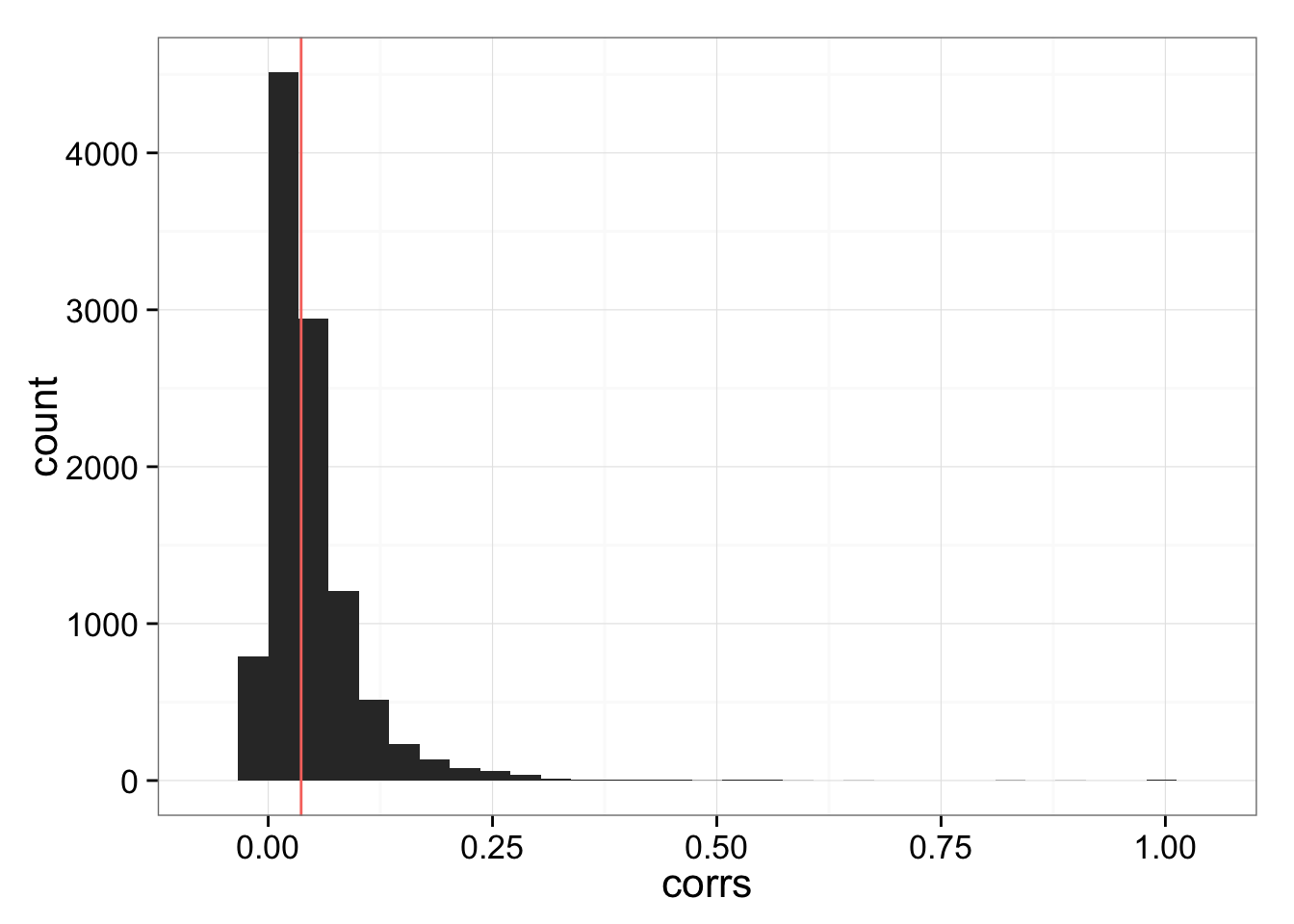

Gene-wise correction

if (file.exists("../data/limma-crossed-per-gene.rda")) {
  load("../data/limma-crossed-per-gene.rda")
} else {
  gls_fit_per_gene <- Humanzee::ruv_mixed_model(molecules_cpm_trans,
                          ndups = 1,
                          per_gene = FALSE,
                          design = design, block = block,
                          correlation = corrs_vec)
  save(gls_fit_per_gene, file = "../data/limma-crossed-per-gene.rda")
}

Compute expression levels after removing variation due to random effects.

molecules_final_per_gene <- t( design %*% t(gls_fit_per_gene$coef) ) + gls_fit_per_gene$resid

pca_final_per_gene <- run_pca(molecules_final_per_gene)
pca_final_plot_per_gene <- plot_pca(pca_final_per_gene$PCs, explained = pca_final_per_gene$explained,
         metadata = anno_filter, color = "individual",
         shape = "replicate") +
  labs(title = "Molecules (batch corrected) for single cells")
pca_final_plot_per_gene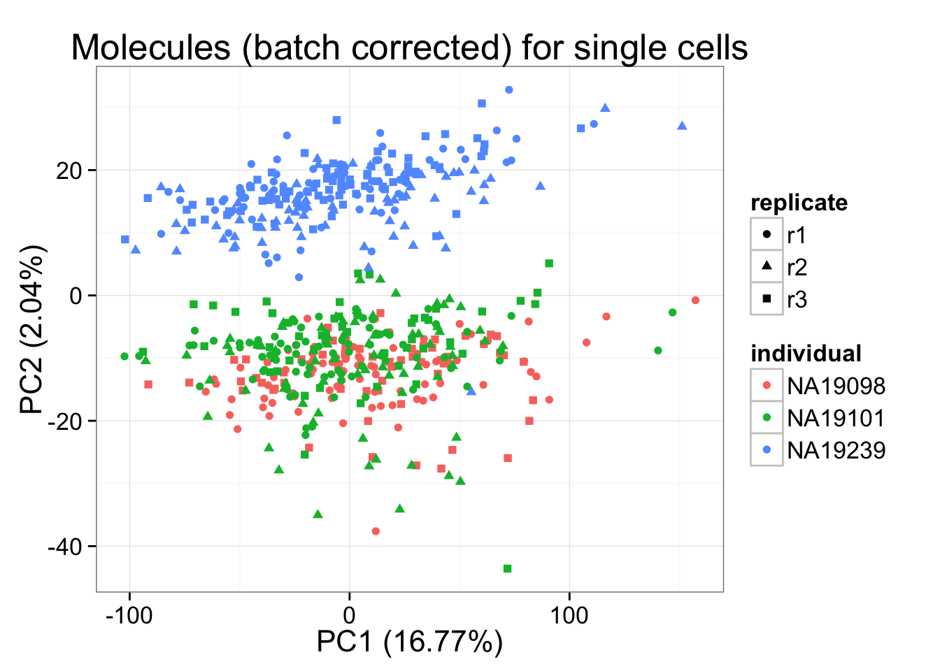

Gene-wide correction

if (file.exists("../data/limma-crossed.rda")) {
  load("../data/limma-crossed.rda")
} else {
  gls_fit <- Humanzee::ruv_mixed_model(molecules_cpm_trans,
                          ndups = 1,
                          per_gene = FALSE,
                          design = design, block = block,
                          correlation = dup_corrs$cor)
  save(gls_fit, file = "../data/limma-crossed.rda")
}

Compute expression levels after removing variation due to random effects.

molecules_final <- t( design %*% t(gls_fit$coef) ) + gls_fit$resid

pca_final <- run_pca(molecules_final)
pca_final_plot <- plot_pca(pca_final$PCs, explained = pca_final$explained,
         metadata = anno_filter, color = "individual",
         shape = "replicate") +
  labs(title = "Molecules (batch corrected) for single cells")
pca_final_plot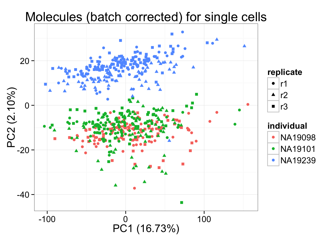

Expression ranking

*Gene ranks per cell are consistent between the gene-wise correction and the gene-wide correction methods. There seems to be more fluctuations in the correlation between the two methods in cell ranks per gene, which suggests a possible impact on the analysis comparing coefficients of variations between genes.

Per-cell correlation in expression levels

cell_corr <- sapply(1:NCOL(molecules_final), function(ii_cell) {
  cor(molecules_final[ , ii_cell], 
      molecules_final_per_gene[ , ii_cell], method = "spearman")
})
summary(cell_corr)

   Min. 1st Qu.  Median    Mean 3rd Qu.    Max. 
 0.9665  0.9958  0.9968  0.9964  0.9977  0.9992

Per-gene correlation in expression levels

gene_corr <- sapply(1:NROW(molecules_final), function(ii_gene) {
  cor(molecules_final[ii_gene, ], 
      molecules_final_per_gene[ii_gene, ], method = "spearman")
})
summary(gene_corr)

   Min. 1st Qu.  Median    Mean 3rd Qu.    Max. 
 0.6550  0.9972  0.9990  0.9974  0.9998  1.0000

Per-gene correlation in expression levels for each individual

gene_corr_individual <- lapply(1:3, function(ii_individual) {
  which_individual <- anno_filter$individual == unique(anno_filter$individual)[ii_individual]
  df <- molecules_final[ , which_individual]
  df_per_gene <- molecules_final_per_gene[ , which_individual]
  cell_corr <- sapply(1:NROW(molecules_final), function(ii_gene) {
          cor(df[ ii_gene, ], 
              df_per_gene[ ii_gene, ], method = "spearman")
        })
  cell_corr
})
lapply(gene_corr_individual, summary)

[[1]]
   Min. 1st Qu.  Median    Mean 3rd Qu.    Max. 
 0.7182  0.9974  0.9991  0.9973  0.9997  1.0000 

[[2]]
   Min. 1st Qu.  Median    Mean 3rd Qu.    Max. 
 0.8431  0.9969  0.9989  0.9971  0.9997  1.0000 

[[3]]
   Min. 1st Qu.  Median    Mean 3rd Qu.    Max. 
 0.5158  0.9972  0.9990  0.9971  0.9997  1.0000

Session information

sessionInfo()

R version 3.2.1 (2015-06-18)
Platform: x86_64-apple-darwin13.4.0 (64-bit)
Running under: OS X 10.10.5 (Yosemite)

locale:
[1] en_US.UTF-8/en_US.UTF-8/en_US.UTF-8/C/en_US.UTF-8/en_US.UTF-8

attached base packages:
[1] stats     graphics  grDevices utils     datasets  methods   base     

other attached packages:
[1] testit_0.4     Humanzee_0.1.0 ggplot2_1.0.1  edgeR_3.10.5  
[5] limma_3.24.15  knitr_1.11    

loaded via a namespace (and not attached):
 [1] Rcpp_0.12.2      magrittr_1.5     MASS_7.3-45      munsell_0.4.2   
 [5] colorspace_1.2-6 stringr_1.0.0    plyr_1.8.3       tools_3.2.1     
 [9] grid_3.2.1       gtable_0.1.2     htmltools_0.2.6  yaml_2.1.13     
[13] digest_0.6.8     reshape2_1.4.1   formatR_1.2.1    evaluate_0.8    
[17] rmarkdown_0.8.1  labeling_0.3     stringi_1.0-1    scales_0.3.0    
[21] proto_0.3-10

Mixed effect model for batch correction - limma

Joyce Hsiao

2015-11-11