Coverage of endogenous genes - bulk reads
2015-02-23
Last updated: 2016-02-23
Code version: 70509eb9a08ffe0fe459efc9de23d89ec424fe99
The sequencing coverage from the UMI protocol should show a very strong 5’ bias. Do we observe this in our data? Here we explore this in a few samples using the genomation package. Specifically, we calculate the mean coverage across all the genes that passed our expression filters for two regions:
- The transcription start site (TSS) +/- 1 kb
- The transcription end site (TES) +/- 1 kb
Using the reads from the bulk samples, we observe the same pattern as with the single cell molecules and reads.
library("genomation")
library("Rsamtools")
library("plyr")
library("tidyr")
library("ggplot2")
theme_set(theme_bw(base_size = 14))
theme_update(panel.grid.minor.x = element_blank(),
             panel.grid.minor.y = element_blank(),
             panel.grid.major.x = element_blank(),
             panel.grid.major.y = element_blank())
Input
Input filtered read counts for bulk samples.
reads_bulk_filter <- read.table("../data/reads-bulk-filter.txt", header = TRUE,
                               stringsAsFactors = FALSE)
Prepare bam files from bulk samples
To investigate the coverage in the bulk samples, we use the first bulk replicate from each individual. Combined reads files for the bulk samples are not available because they are unnecessary for the pipeline. Since each per lane bam file has many sequences, we will choose an arbitrary lane.
bulk_lanes <- c("19098.1.bulk.GCTGAGGT.L001.R1.C6WYKACXX",
                "19101.1.bulk.GGATACGT.L001.R1.C6WYKACXX",
                "19239.1.bulk.ACAGCGAA.L001.R1.C6WYKACXX")
From the sequencing pipeline, the per lane bam files for the bulk reads are in bam-processed and have the filename structure individual.replicate.well.index.lane.R1.flowcell.trim.sickle.sorted.bam. These files are already sorted and indexed.
bam_reads <- paste0(bulk_lanes, ".trim.sickle.sorted.bam")
data_dir <- "/mnt/gluster/home/jdblischak/ssd"
from_file <- file.path(data_dir, "bam-processed", bam_reads)
to_file <- file.path("../data", bam_reads)
indexed_file <- paste0(bam_reads, ".bai")
from_file_index <- file.path(data_dir, "bam-processed", indexed_file)
to_file_index <- file.path("../data", indexed_file)
for (f in 1:length(bam_reads)) {
  if (!file.exists(to_file_index[f])) {
    stopifnot(file.exists(from_file[f], from_file_index[f]))
    file.copy(from_file[f], to_file[f])
    file.copy(from_file_index[f], to_file_index[f])
  }
}
stopifnot(file.exists(to_file, to_file_index))
bam <- to_file
bam
[1] "../data/19098.1.bulk.GCTGAGGT.L001.R1.C6WYKACXX.trim.sickle.sorted.bam"
[2] "../data/19101.1.bulk.GGATACGT.L001.R1.C6WYKACXX.trim.sickle.sorted.bam"
[3] "../data/19239.1.bulk.ACAGCGAA.L001.R1.C6WYKACXX.trim.sickle.sorted.bam"Prepare genomic features
The genomic features are created with the script create-transcripts.R.
Input transcription start sites (TSS).
tss <- readBed("../data/tss.bed")
tss <- tss[tss$name %in% rownames(reads_bulk_filter)]
Input transcription end sites (TES).
tes <- readBed("../data/tes.bed")
tes <- tes[tes$name %in% rownames(reads_bulk_filter)]
Calculate coverage over genomic features
TSS
tss_sm = ScoreMatrixList(target = bam, windows = tss, type = "bam",
                         rpm = TRUE, strand.aware = TRUE)
working on: 19098.1.bulk.GCTGAGGT.L001.R1.C6WYKACXX.trim.sickle.sorted.bam
Normalizing to rpm ...
working on: 19101.1.bulk.GGATACGT.L001.R1.C6WYKACXX.trim.sickle.sorted.bam
Normalizing to rpm ...
working on: 19239.1.bulk.ACAGCGAA.L001.R1.C6WYKACXX.trim.sickle.sorted.bam
Normalizing to rpm ...tss_smscoreMatrixlist of length:3
1. scoreMatrix with dims: 12192 2001
2. scoreMatrix with dims: 12192 2001
3. scoreMatrix with dims: 12192 2001TES
tes_sm = ScoreMatrixList(target = bam, windows = tes, type = "bam",
                         rpm = TRUE, strand.aware = TRUE)
working on: 19098.1.bulk.GCTGAGGT.L001.R1.C6WYKACXX.trim.sickle.sorted.bam
Normalizing to rpm ...
working on: 19101.1.bulk.GGATACGT.L001.R1.C6WYKACXX.trim.sickle.sorted.bam
Normalizing to rpm ...
working on: 19239.1.bulk.ACAGCGAA.L001.R1.C6WYKACXX.trim.sickle.sorted.bam
Normalizing to rpm ...tes_smscoreMatrixlist of length:3
1. scoreMatrix with dims: 12191 2001
2. scoreMatrix with dims: 12191 2001
3. scoreMatrix with dims: 12191 2001Summarize coverage
Calculate the mean coverage per base pair for the TSS and and TES.
names(tss_sm) <- bulk_lanes
tss_sm_df <- ldply(tss_sm, colMeans, .id = "sample_id")
colnames(tss_sm_df)[-1] <- paste0("p", 1:(ncol(tss_sm_df) - 1))
tss_sm_df$feature = "TSS"
tss_sm_df_long <- gather(tss_sm_df, key = "pos", value = "rpm", p1:p2001)
names(tes_sm) <- bulk_lanes
tes_sm_df <- ldply(tes_sm, colMeans, .id = "sample_id")
colnames(tes_sm_df)[-1] <- paste0("p", 1:(ncol(tes_sm_df) - 1))
tes_sm_df$feature = "TES"
tes_sm_df_long <- gather(tes_sm_df, key = "pos", value = "rpm", p1:p2001)Combine the two features.
features <- rbind(tss_sm_df_long, tes_sm_df_long)
# Convert base position back to integer value
features$pos <- sub("p", "", features$pos)
features$pos <- as.numeric(features$pos)
# Subtract 1001 to recalibrate as +/- 1 kb
features$pos <- features$pos - 1001
# Order factor so that TSS is displayed left of TES
features$feature <- factor(features$feature, levels = c("TSS", "TES"),
                           labels = c("Transcription start site",
                                      "Transription end site"))
Metagene plot
ggplot(features, aes(x = pos, y = rpm, color = sample_id)) +
  geom_line() +
  facet_wrap(~feature) +
  scale_color_discrete(name = "Sample") +
  labs(x = "Relative position (bp)",
       y = "Counts per million (mean)",
       title = "5' bias of UMI protocol") +
  theme(legend.position = "bottom",
        legend.text = element_text(size = 6))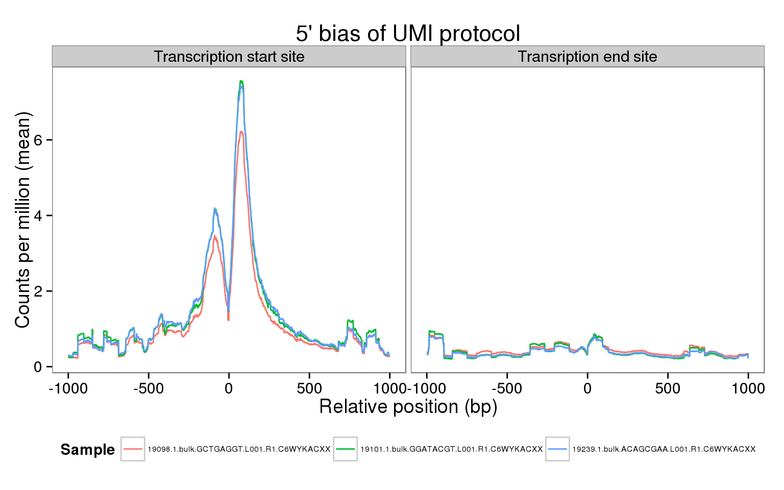
Interpretation
These results are similar to those obtained using the single cell molecules and reads. Furthermore, they have many more reads and thus do not suffer as much from sparsity.
Session information
sessionInfo()R version 3.2.0 (2015-04-16)
Platform: x86_64-unknown-linux-gnu (64-bit)
locale:
[1] LC_CTYPE=en_US.UTF-8 LC_NUMERIC=C
[3] LC_TIME=en_US.UTF-8 LC_COLLATE=en_US.UTF-8
[5] LC_MONETARY=en_US.UTF-8 LC_MESSAGES=en_US.UTF-8
[7] LC_PAPER=en_US.UTF-8 LC_NAME=C
[9] LC_ADDRESS=C LC_TELEPHONE=C
[11] LC_MEASUREMENT=en_US.UTF-8 LC_IDENTIFICATION=C
attached base packages:
[1] parallel stats4 grid stats graphics grDevices utils
[8] datasets methods base
other attached packages:
[1] ggplot2_1.0.1 tidyr_0.2.0 plyr_1.8.3
[4] Rsamtools_1.20.4 Biostrings_2.36.1 XVector_0.8.0
[7] GenomicRanges_1.20.5 GenomeInfoDb_1.4.0 IRanges_2.2.4
[10] S4Vectors_0.6.0 BiocGenerics_0.14.0 genomation_1.0.0
[13] knitr_1.10.5
loaded via a namespace (and not attached):
[1] Rcpp_0.12.0 formatR_1.2
[3] futile.logger_1.4.1 bitops_1.0-6
[5] futile.options_1.0.0 tools_3.2.0
[7] zlibbioc_1.14.0 digest_0.6.8
[9] evaluate_0.7 gtable_0.1.2
[11] gridBase_0.4-7 DBI_0.3.1
[13] yaml_2.1.13 proto_0.3-10
[15] dplyr_0.4.2 rtracklayer_1.28.4
[17] httr_0.6.1 stringr_1.0.0
[19] data.table_1.9.4 impute_1.42.0
[21] R6_2.1.1 XML_3.98-1.2
[23] BiocParallel_1.2.2 rmarkdown_0.6.1
[25] reshape2_1.4.1 lambda.r_1.1.7
[27] magrittr_1.5 codetools_0.2-11
[29] scales_0.2.4 htmltools_0.2.6
[31] GenomicAlignments_1.4.1 MASS_7.3-40
[33] assertthat_0.1 colorspace_1.2-6
[35] labeling_0.3 stringi_0.4-1
[37] lazyeval_0.1.10 RCurl_1.95-4.6
[39] munsell_0.4.2 chron_2.3-45