Profile individual adjusted CVs
Joyce Hsiao
2015-10-29
Last updated: 2015-12-11
Code version: 884b335605607bd2cf5c9a1ada1e345466388866
Objective
We computed the adjusted CV for each individual and observed that genes with extreme CVs are unique to each individual, while genes with extreme means are likey to be shared across individuals. Moreover, the extreme genes are not more likely to be cell cycle genes than the non-extreme genes; in fact, we can see from the scatter plots that cell cycle genes tend to be small in our adjusted CV than the non-cell-cycle genes.
Set up
library("data.table")
library("dplyr")
library("limma")
library("edgeR")
library("ggplot2")
library("grid")
theme_set(theme_bw(base_size = 12))
source("functions.R")
Prepare data
Input annotation of only QC-filtered single cells. Remove NA19098.r2
anno_qc <- read.table("../data/annotation-filter.txt", header = TRUE,
                   stringsAsFactors = FALSE)
is_include <- anno_qc$batch != "NA19098.r2"
anno_qc_filter <- anno_qc[which(is_include), ]
Import endogeneous gene molecule counts that are QC-filtered, CPM-normalized, ERCC-normalized, and also processed to remove unwanted variation from batch effet. ERCC genes are removed from this file.
molecules_ENSG <- read.table("../data/molecules-final.txt", header = TRUE, stringsAsFactors = FALSE)
molecules_ENSG <- molecules_ENSG[ , is_include]
Input moleclule counts before log2 CPM transformation. This file is used to compute percent zero-count cells per sample.
molecules_sparse <- read.table("../data/molecules-filter.txt", header = TRUE, stringsAsFactors = FALSE)

molecules_sparse <- molecules_sparse[grep("ENSG", rownames(molecules_sparse)), ]
stopifnot( all.equal(rownames(molecules_ENSG), rownames(molecules_sparse)) )
Compute normalized CV
We compute squared CV across cells for each individual and then for each individual CV profile, account for mean dependency by computing distance with respect to the data-wide coefficient variation on the log10 scale.
source("../code/cv-functions.r")

ENSG_cv <- compute_cv(log2counts = molecules_ENSG,
                      grouping_vector = anno_qc_filter$individual)

ENSG_cv_adj <- normalize_cv(group_cv = ENSG_cv,
                            log2counts = molecules_ENSG,
                            anno = anno_qc_filter)
*Some plotting
Mark genes with black dots if log10(cv^2) > .5.
Distance to the data-wise CV (adjusted CV): small CV values are more variable in terms their distance to the data-wise CV value; hence we see a large distance to the data-wise CV for the small CVs than the large CVs.
high_cv <- subset(do.call(rbind, ENSG_cv_adj), log10(cv^2) > .5)
ggplot(do.call(rbind, ENSG_cv_adj),
       aes(x = log10(mean), y = log10(cv^2))) +
  geom_point(aes(col = group)) + facet_wrap( ~ group) +
  ggtitle("CV-mean relationship") +
  geom_point(data = high_cv, colour = "black")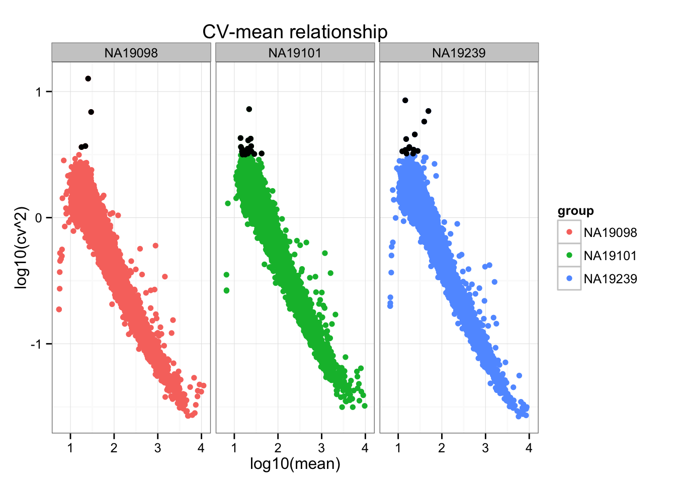
ggplot(do.call(rbind, ENSG_cv_adj),
       aes(x = log10(mean), y = log10cv2_adj)) +
  geom_point(aes(col = group)) + facet_wrap( ~ group) +
  ggtitle("Adjusted CV and mean relationship") +
  geom_point(data = high_cv, colour = "black")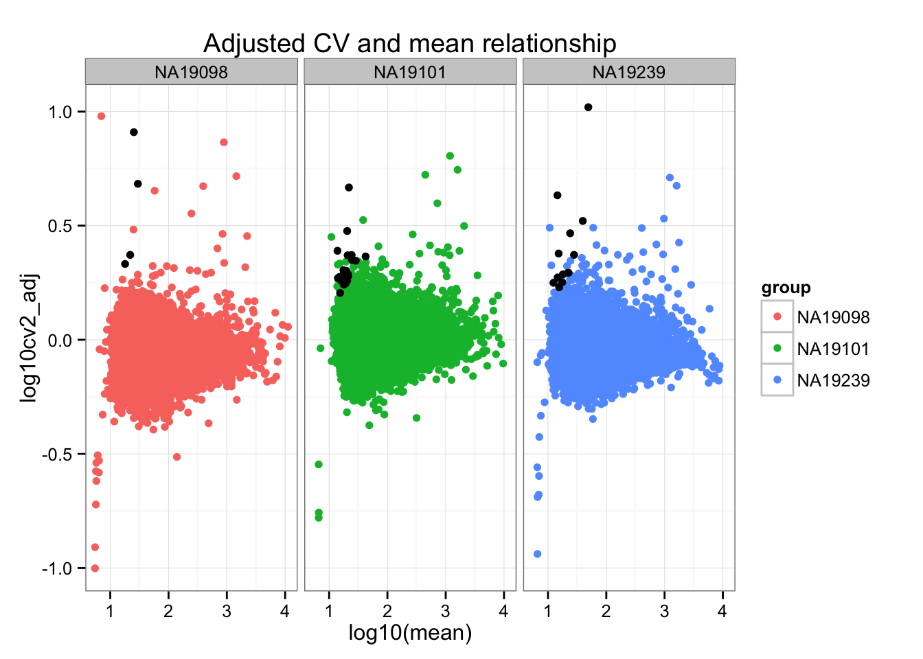
ggplot(do.call(rbind, ENSG_cv_adj),
       aes(x = log10(cv^2), y = log10cv2_adj)) +
  geom_point(aes(col = group)) + facet_wrap( ~ group) +
  ggtitle("CV before versus after adjustment") +
  geom_point(data = high_cv, colour = "black")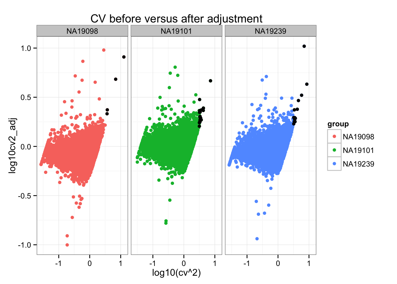
Gene ranks venn diagrams
Extreme genes as in top/bottom 50
extreme_genes_50 <- lapply(ENSG_cv_adj, function(xx) {
  low_mean <- rank(xx$mean) < 50
  high_mean <- rank(xx$mean) > (length(xx$mean) - 50)
  low_cv <-  rank(xx$log10cv2_adj) < 50
  high_cv <- rank(xx$log10cv2_adj) > (length(xx$log10cv2_adj) - 50)
  res <- data.frame(high_mean = high_mean,
                    low_mean = low_mean,
                    high_cv = high_cv,
                    low_cv = low_cv)
  rownames(res) <- rownames(ENSG_cv_adj[[1]])
  res
})
*Top 50 in adjusted CV
genes <- rownames(extreme_genes_50[[1]])
library(gplots)
venn( list(genes[extreme_genes_50[[1]]$high_cv],
            genes[extreme_genes_50[[2]]$high_cv],
            genes[extreme_genes_50[[3]]$high_cv] ) )
*Bottom 50 in adjusted CV
genes <- rownames(extreme_genes_50[[1]])
library(gplots)
venn( list(genes[extreme_genes_50[[1]]$low_cv],
            genes[extreme_genes_50[[2]]$low_cv],
            genes[extreme_genes_50[[3]]$low_cv] ) )
*Top 50 in mean
genes <- rownames(extreme_genes_50[[1]])
library(gplots)
venn( list(genes[extreme_genes_50[[1]]$high_mean],
            genes[extreme_genes_50[[2]]$high_mean],
            genes[extreme_genes_50[[3]]$high_mean] ) )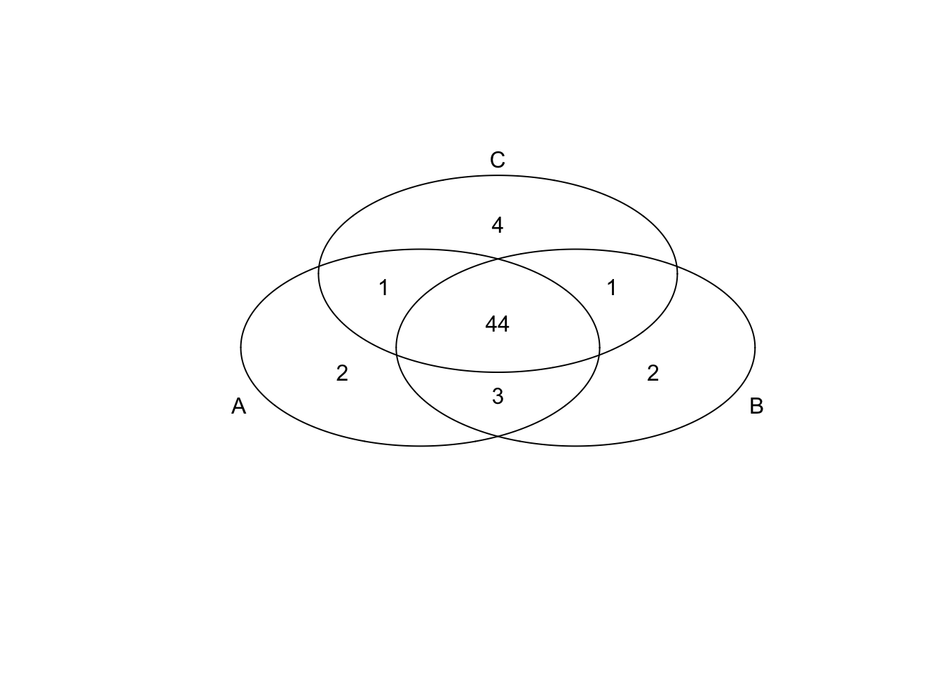
*Bottom 50 in mean
genes <- rownames(extreme_genes_50[[1]])
library(gplots)
venn( list(genes[extreme_genes_50[[1]]$low_mean],
            genes[extreme_genes_50[[2]]$low_mean],
            genes[extreme_genes_50[[3]]$low_mean] ) )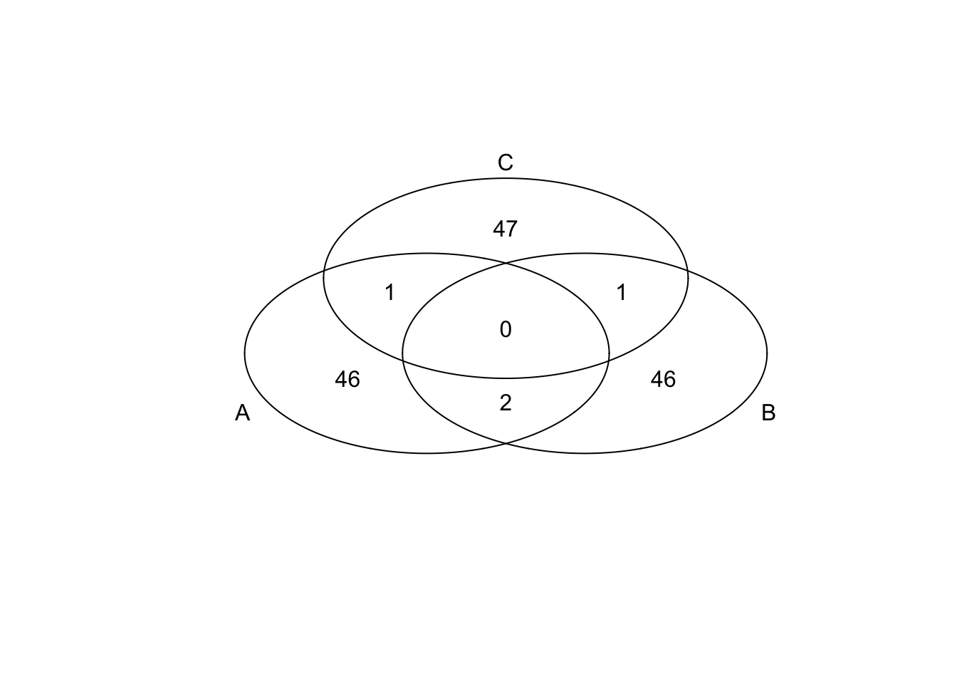
Extreme genes as in top/bottom 200
extreme_genes_200 <- lapply(ENSG_cv_adj, function(xx) {
  low_mean <- rank(xx$mean) < 200
  high_mean <- rank(xx$mean) > (length(xx$mean) - 200)
  low_cv <-  rank(xx$log10cv2_adj) < 200
  high_cv <- rank(xx$log10cv2_adj) > (length(xx$log10cv2_adj) - 200)
  res <- data.frame(high_mean = high_mean,
                    low_mean = low_mean,
                    high_cv = high_cv,
                    low_cv = low_cv)
  rownames(res) <- rownames(ENSG_cv_adj[[1]])
  res
})
*Top 200 in adjusted CV
genes <- rownames(extreme_genes_200[[1]])
library(gplots)
venn( list(genes[extreme_genes_200[[1]]$high_cv],
            genes[extreme_genes_200[[2]]$high_cv],
            genes[extreme_genes_200[[3]]$high_cv] ) )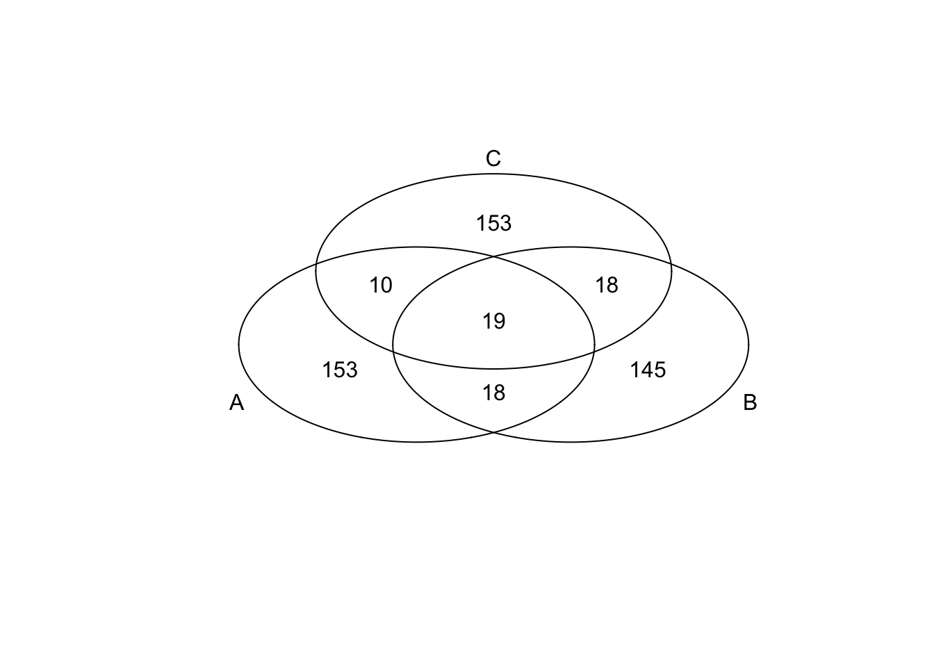
*Bottom 200 in adjusted CV
genes <- rownames(extreme_genes_200[[1]])
library(gplots)
venn( list(genes[extreme_genes_200[[1]]$low_cv],
            genes[extreme_genes_200[[2]]$low_cv],
            genes[extreme_genes_200[[3]]$low_cv] ) )
*Top 200 in mean
genes <- rownames(extreme_genes_200[[1]])
library(gplots)
venn( list(genes[extreme_genes_200[[1]]$high_mean],
            genes[extreme_genes_200[[2]]$high_mean],
            genes[extreme_genes_200[[3]]$high_mean] ) )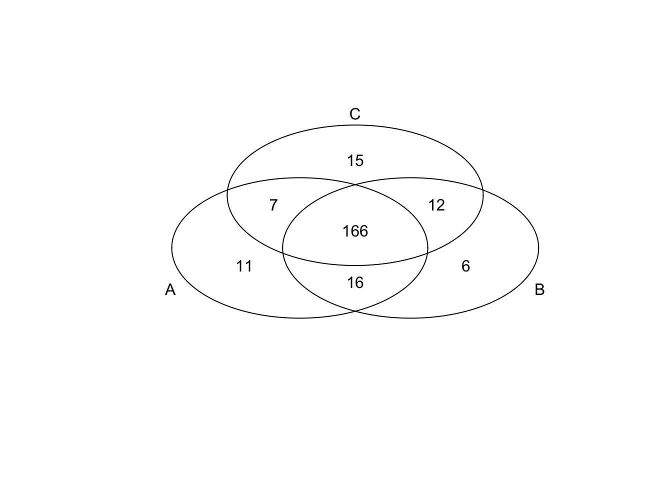
*Extreme genes as in top/bottom 500
extreme_genes_500 <- lapply(ENSG_cv_adj, function(xx) {
  low_mean <- rank(xx$mean) < 500
  high_mean <- rank(xx$mean) > (length(xx$mean) - 500)
  low_cv <-  rank(xx$log10cv2_adj) < 500
  high_cv <- rank(xx$log10cv2_adj) > (length(xx$log10cv2_adj) - 500)
  res <- data.frame(high_mean = high_mean,
                    low_mean = low_mean,
                    high_cv = high_cv,
                    low_cv = low_cv)
  rownames(res) <- rownames(ENSG_cv_adj[[1]])
  res
})
*Top 500 in adjusted CV
genes <- rownames(extreme_genes_500[[1]])
library(gplots)
venn( list(genes[extreme_genes_500[[1]]$high_cv],
            genes[extreme_genes_500[[2]]$high_cv],
            genes[extreme_genes_500[[3]]$high_cv] ) )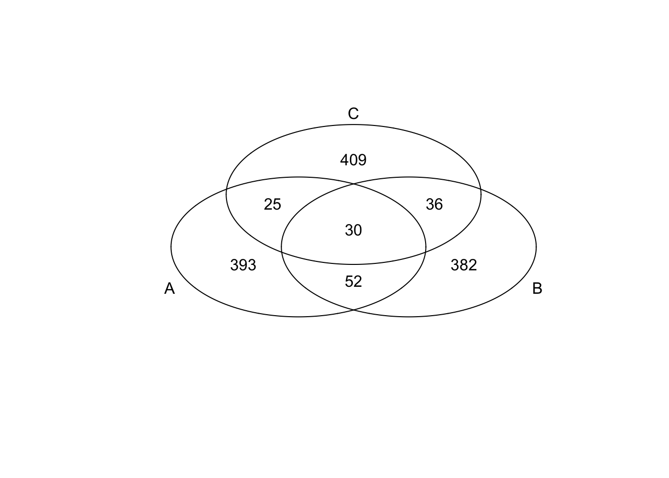
*Bottom 200 in adjusted CV
genes <- rownames(extreme_genes_500[[1]])
library(gplots)
venn( list(genes[extreme_genes_500[[1]]$low_cv],
            genes[extreme_genes_500[[2]]$low_cv],
            genes[extreme_genes_500[[3]]$low_cv] ) )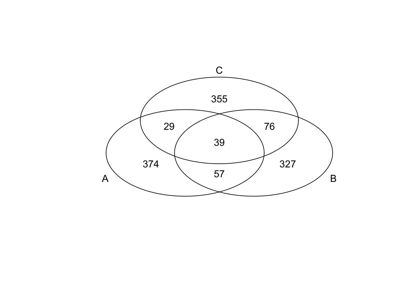
*Top 200 in mean
genes <- rownames(extreme_genes_500[[1]])
library(gplots)
venn( list(genes[extreme_genes_500[[1]]$high_mean],
            genes[extreme_genes_500[[2]]$high_mean],
            genes[extreme_genes_500[[3]]$high_mean] ) )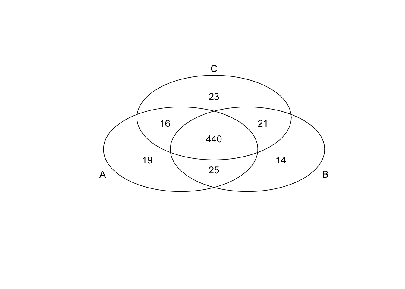
*Bottom 200 in mean
genes <- rownames(extreme_genes_500[[1]])
library(gplots)
venn( list(genes[extreme_genes_500[[1]]$low_mean],
            genes[extreme_genes_500[[2]]$low_mean],
            genes[extreme_genes_500[[3]]$low_mean] ) )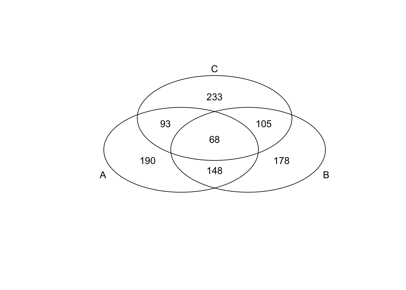
Gene ranks plot
*Top 50 in adjusted CV
ggplot(do.call(rbind, ENSG_cv_adj),
       aes(x = log10(mean), y = log10cv2_adj)) +
  geom_point(aes(col = group), cex = .8) + facet_wrap( ~ group) +
  ggtitle("Adj-CV top 50, NA19098") +
  geom_point(data = subset(do.call(rbind, ENSG_cv_adj), extreme_genes_50[[1]]$high_cv),
             colour = "grey20")
ggplot(do.call(rbind, ENSG_cv_adj),
       aes(x = log10(mean), y = log10cv2_adj)) +
  geom_point(aes(col = group), cex = .8) + facet_wrap( ~ group) +
  ggtitle("Adj-CV top 50, NA19101") +
  geom_point(data = subset(do.call(rbind, ENSG_cv_adj), extreme_genes_50[[2]]$high_cv),
             colour = "grey20")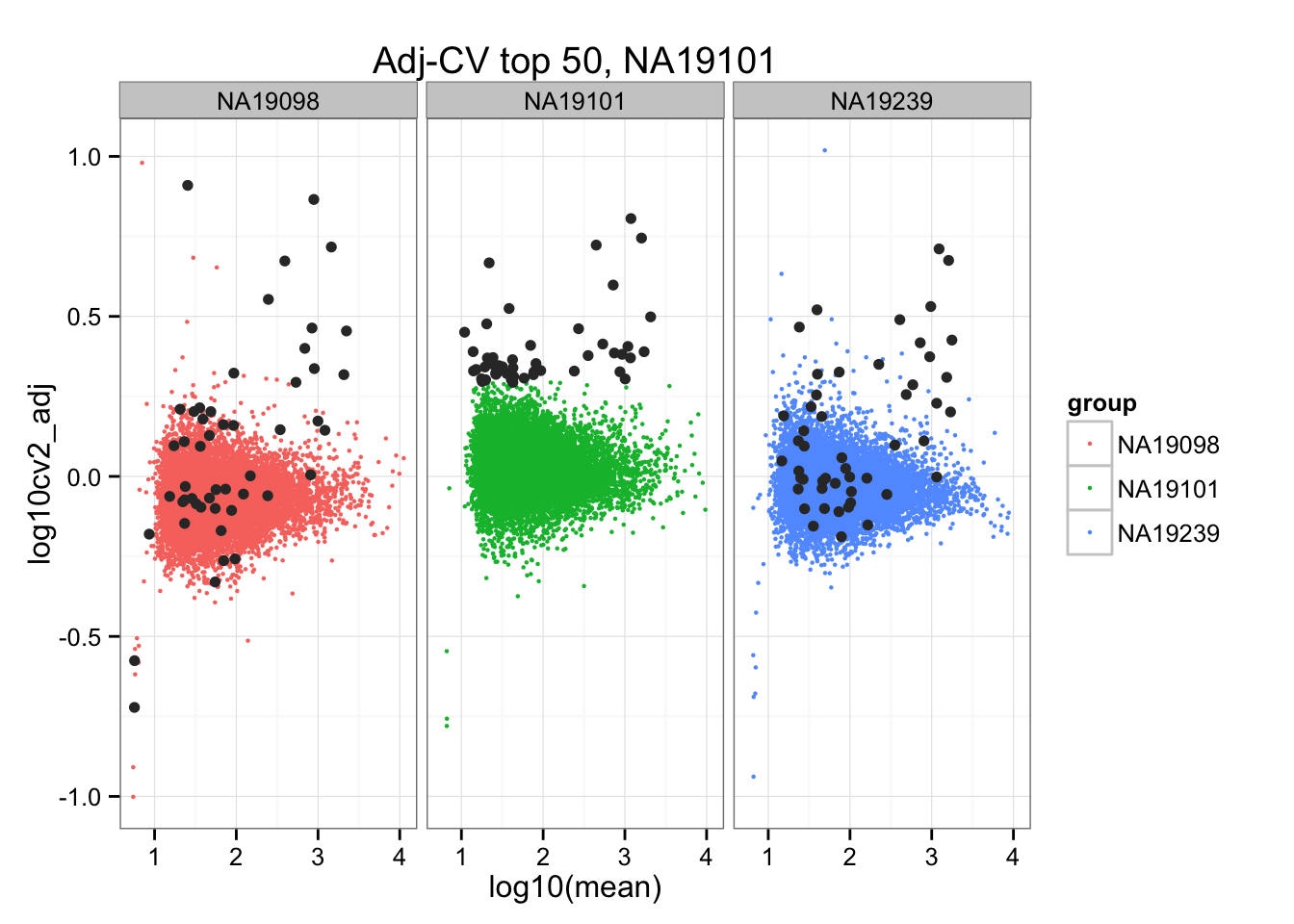
ggplot(do.call(rbind, ENSG_cv_adj),
       aes(x = log10(mean), y = log10cv2_adj)) +
  geom_point(aes(col = group), cex = .8) + facet_wrap( ~ group) +
  ggtitle("Adj-CV top 50, NA19239") +
  geom_point(data = subset(do.call(rbind, ENSG_cv_adj), extreme_genes_50[[3]]$high_cv),
             colour = "grey20")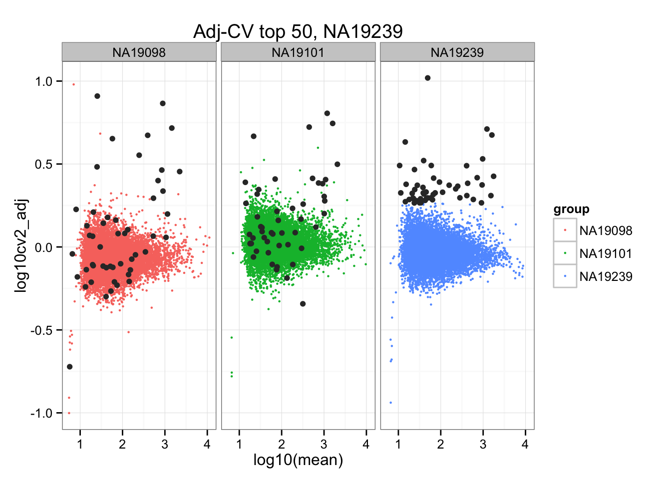
*Top 200 in adjusted CV
ggplot(do.call(rbind, ENSG_cv_adj),
       aes(x = log10(mean), y = log10cv2_adj)) +
  geom_point(aes(col = group), cex = .8) + facet_wrap( ~ group) +
  ggtitle("Adj-CV top 50, NA19098") +
  geom_point(data = subset(do.call(rbind, ENSG_cv_adj), extreme_genes_200[[1]]$high_cv),
             colour = "grey20")
ggplot(do.call(rbind, ENSG_cv_adj),
       aes(x = log10(mean), y = log10cv2_adj)) +
  geom_point(aes(col = group), cex = .8) + facet_wrap( ~ group) +
  ggtitle("Adj-CV top 50, NA19101") +
  geom_point(data = subset(do.call(rbind, ENSG_cv_adj), extreme_genes_200[[2]]$high_cv),
             colour = "grey20")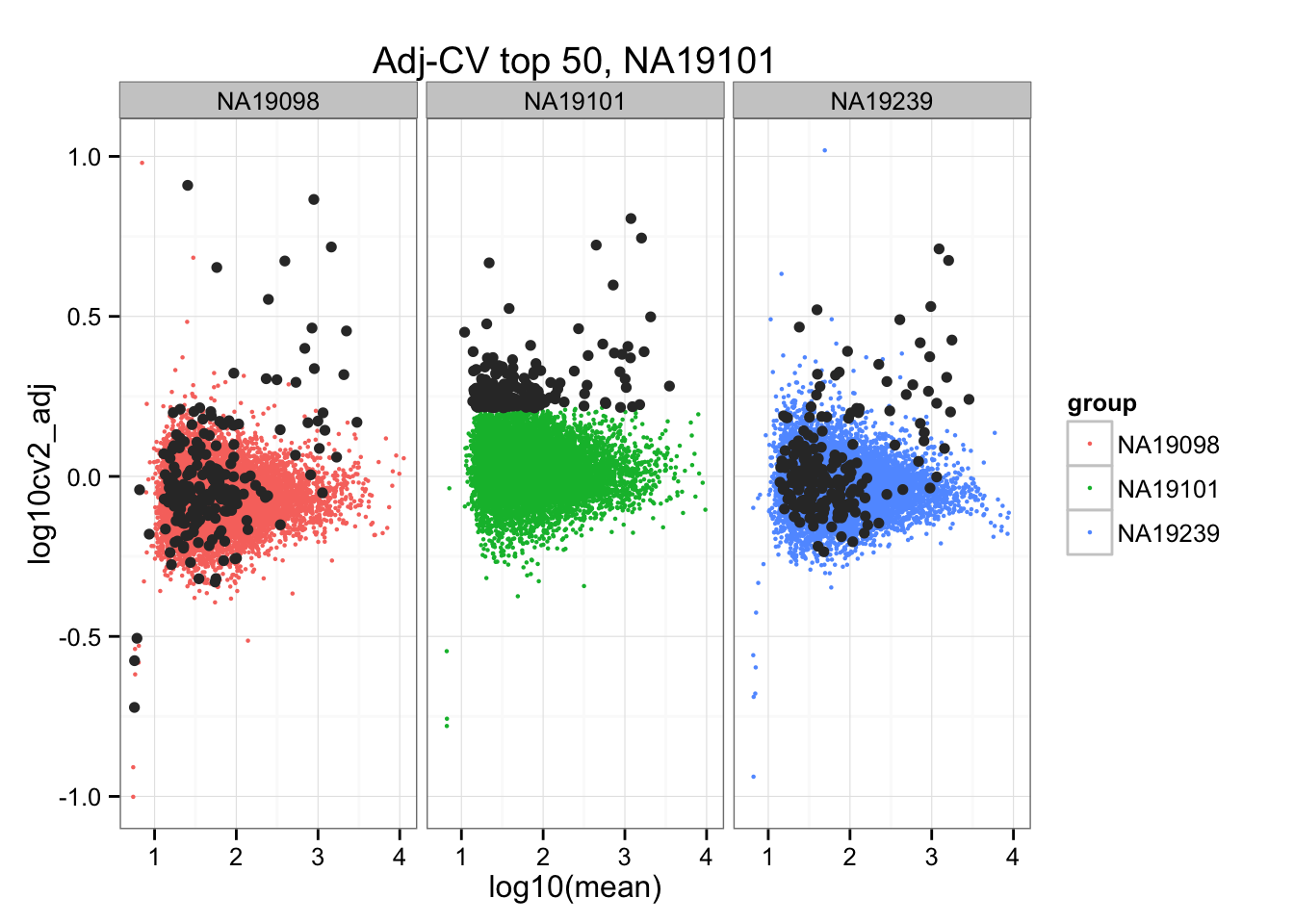
ggplot(do.call(rbind, ENSG_cv_adj),
       aes(x = log10(mean), y = log10cv2_adj)) +
  geom_point(aes(col = group), cex = .8) + facet_wrap( ~ group) +
  ggtitle("Adj-CV top 50, NA19239") +
  geom_point(data = subset(do.call(rbind, ENSG_cv_adj), extreme_genes_200[[3]]$high_cv),
             colour = "grey20")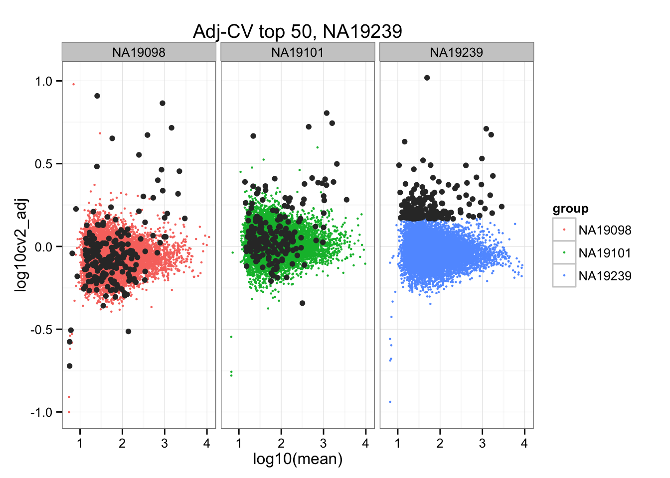
*Bottom 50 in adjusted CV
ggplot(do.call(rbind, ENSG_cv_adj),
       aes(x = log10(mean), y = log10cv2_adj)) +
  geom_point(aes(col = group), cex = .8) + facet_wrap( ~ group) +
  ggtitle("Adj-CV top 50, NA19098") +
  geom_point(data = subset(do.call(rbind, ENSG_cv_adj), extreme_genes_50[[1]]$low_cv),
             colour = "grey20")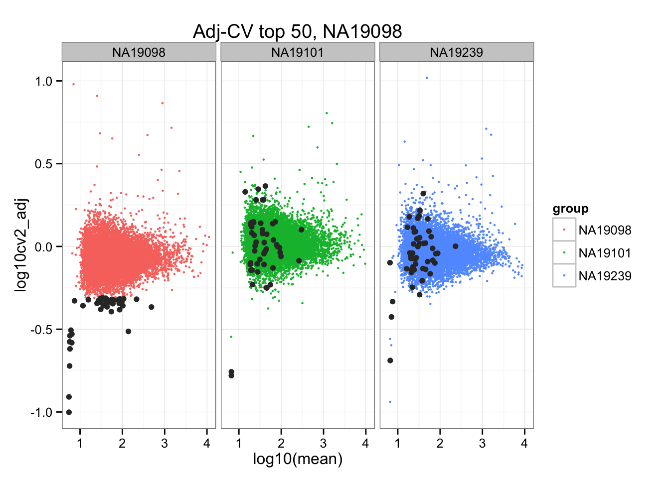
ggplot(do.call(rbind, ENSG_cv_adj),
       aes(x = log10(mean), y = log10cv2_adj)) +
  geom_point(aes(col = group), cex = .8) + facet_wrap( ~ group) +
  ggtitle("Adj-CV top 50, NA19101") +
  geom_point(data = subset(do.call(rbind, ENSG_cv_adj), extreme_genes_50[[2]]$low_cv),
             colour = "grey20")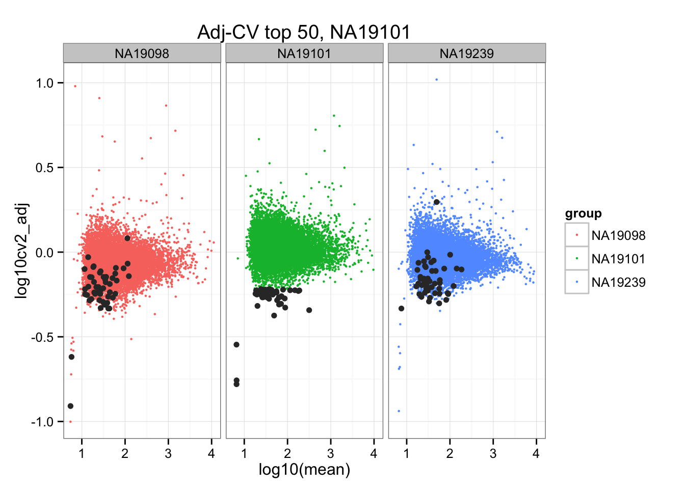
ggplot(do.call(rbind, ENSG_cv_adj),
       aes(x = log10(mean), y = log10cv2_adj)) +
  geom_point(aes(col = group), cex = .8) + facet_wrap( ~ group) +
  ggtitle("Adj-CV top 50, NA19239") +
  geom_point(data = subset(do.call(rbind, ENSG_cv_adj), extreme_genes_50[[3]]$low_cv),
             colour = "grey20")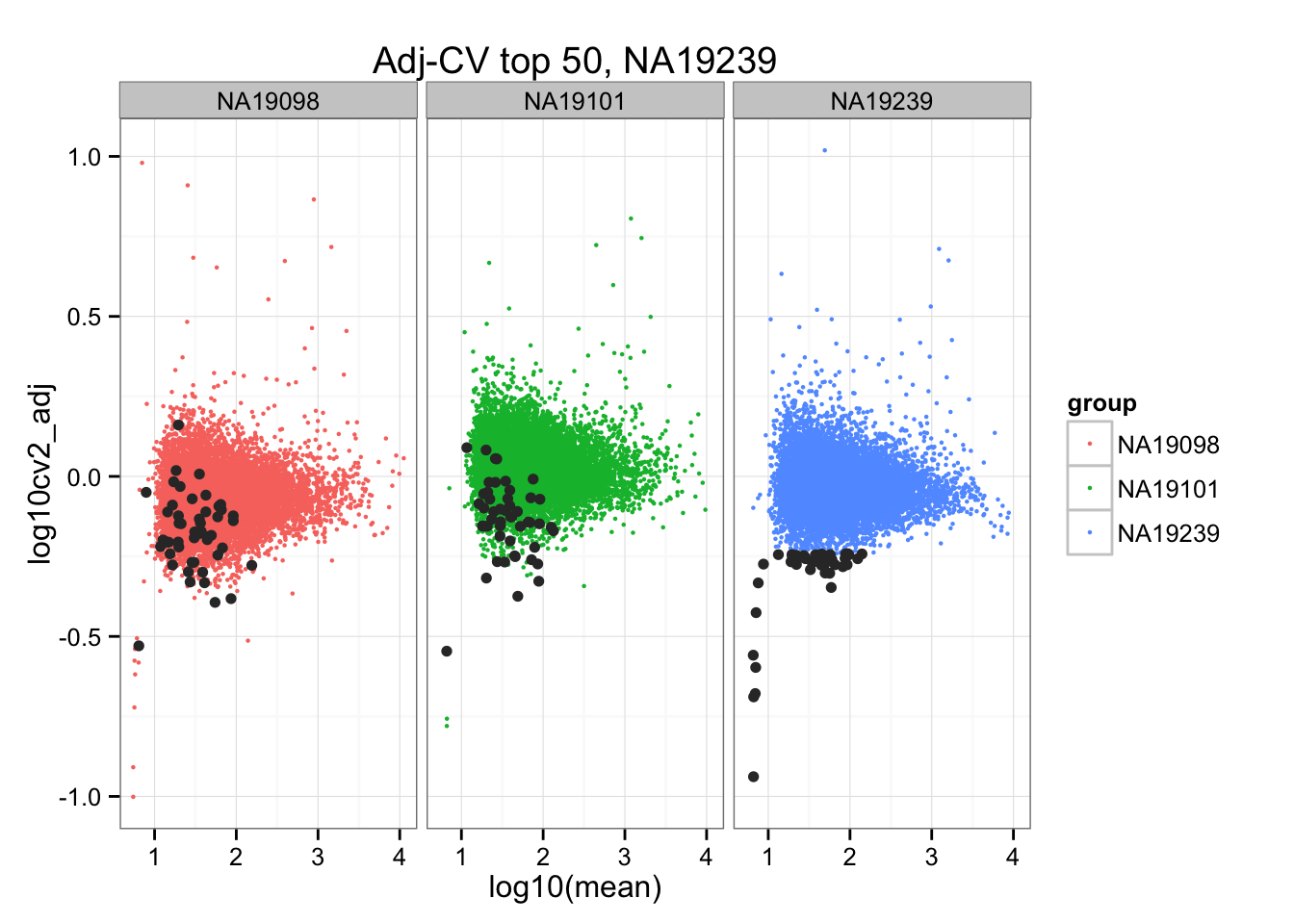
*Bottom 200 in adjusted CV
ggplot(do.call(rbind, ENSG_cv_adj),
       aes(x = log10(mean), y = log10cv2_adj)) +
  geom_point(aes(col = group), cex = .8) + facet_wrap( ~ group) +
  ggtitle("Adj-CV top 50, NA19098") +
  geom_point(data = subset(do.call(rbind, ENSG_cv_adj), extreme_genes_200[[1]]$low_cv),
             colour = "grey20")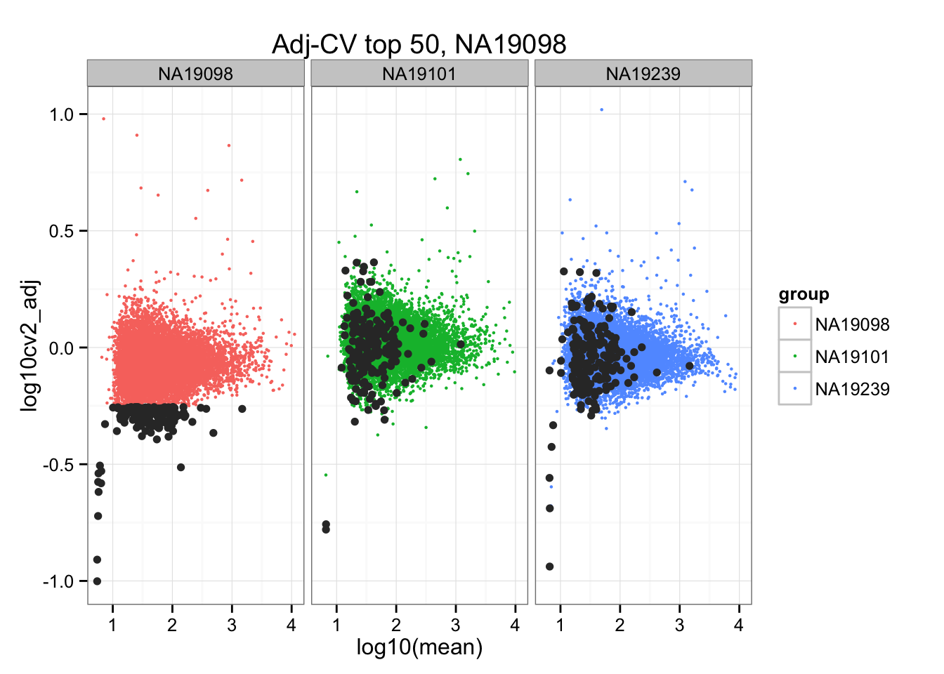
ggplot(do.call(rbind, ENSG_cv_adj),
       aes(x = log10(mean), y = log10cv2_adj)) +
  geom_point(aes(col = group), cex = .8) + facet_wrap( ~ group) +
  ggtitle("Adj-CV top 50, NA19101") +
  geom_point(data = subset(do.call(rbind, ENSG_cv_adj), extreme_genes_200[[2]]$low_cv),
             colour = "grey20")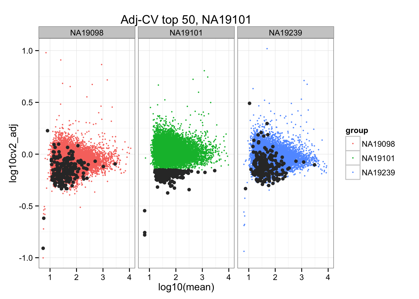
ggplot(do.call(rbind, ENSG_cv_adj),
       aes(x = log10(mean), y = log10cv2_adj)) +
  geom_point(aes(col = group), cex = .8) + facet_wrap( ~ group) +
  ggtitle("Adj-CV top 50, NA19239") +
  geom_point(data = subset(do.call(rbind, ENSG_cv_adj), extreme_genes_200[[3]]$low_cv),
             colour = "grey20")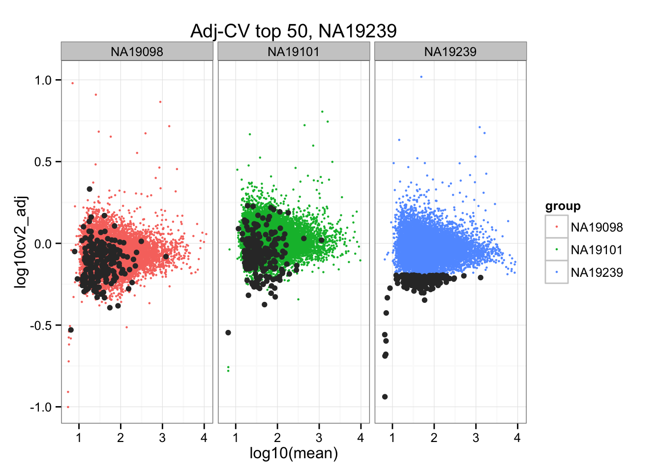
Cell cycle
*Import cell-cycle gene list
cellcycle_genes <- read.table("../data/cellcyclegenes.txt", sep = "\t",
                              header = TRUE, stringsAsFactors = FALSE)
str(cellcycle_genes)
'data.frame': 151 obs. of 5 variables:
$ G1.S: chr "ENSG00000102977" "ENSG00000119640" "ENSG00000154734" "ENSG00000088448" ...
$ S : chr "ENSG00000114770" "ENSG00000144827" "ENSG00000180071" "ENSG00000105011" ...
$ G2.M: chr "ENSG00000011426" "ENSG00000065000" "ENSG00000213390" "ENSG00000122644" ...
$ M : chr "ENSG00000135541" "ENSG00000135334" "ENSG00000154945" "ENSG00000011426" ...
$ M.G1: chr "ENSG00000173744" "ENSG00000160216" "ENSG00000170776" "ENSG00000218624" ...genes <- rownames(extreme_genes_50[[1]])
ii_cellcycle_genes <- lapply(1:3, function(per_individual) {
genes %in% unlist(cellcycle_genes)
})
names(ii_cellcycle_genes) <- names(extreme_genes_50)
ii_cellcycle_genes <- do.call(c, ii_cellcycle_genes)ggplot(do.call(rbind, ENSG_cv_adj),
aes(x = log10(mean), y = log10cv2_adj)) +
geom_point(aes(col = group), cex = 1.2) + facet_wrap( ~ group) +
ggtitle("Cellcycle genes") +
geom_point(data = subset(do.call(rbind, ENSG_cv_adj),
ii_cellcycle_genes),
colour = "grey20", cex = 1.2)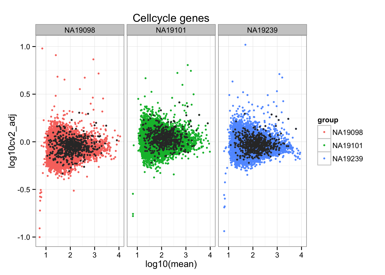
Pluripotent genes
*Import pluripotent gene list
pluripotent_genes <- read.table("../data/pluripotency-genes.txt", sep = "\t",
                              header = TRUE, stringsAsFactors = FALSE)
str(pluripotent_genes)
'data.frame': 27 obs. of 4 variables:
$ From : chr "GDF3" "ZFP42" "NR6A1" "SOX2" ...
$ To : chr "ENSG00000184344" "ENSG00000179059" "ENSG00000148200" "ENSG00000181449" ...
$ Species : chr "Homo sapiens" "Homo sapiens" "Homo sapiens" "Homo sapiens" ...
$ Gene.Name: chr "growth differentiation factor 3" "zinc finger protein 42 homolog (mouse)" "nuclear receptor subfamily 6, group A, member 1" "SRY (sex determining region Y)-box 2" ...genes <- rownames(extreme_genes_50[[1]])
ii_pluripotent_genes <- lapply(1:3, function(per_individual) {
genes %in% unlist(pluripotent_genes$To)
})
names(ii_pluripotent_genes) <- names(extreme_genes_50)
ii_pluripotent_genes <- do.call(c, ii_pluripotent_genes)ggplot(do.call(rbind, ENSG_cv_adj),
aes(x = log10(mean), y = log10cv2_adj)) +
geom_point(aes(col = group), cex = 1.2) + facet_wrap( ~ group) +
ggtitle("Pluripotent genes") +
geom_point(data = subset(do.call(rbind, ENSG_cv_adj),
ii_pluripotent_genes),
colour = "grey20", cex = 1.2)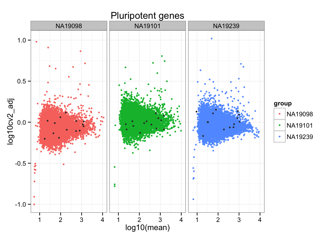
Session information
sessionInfo()R version 3.2.1 (2015-06-18)
Platform: x86_64-apple-darwin13.4.0 (64-bit)
Running under: OS X 10.10.5 (Yosemite)
locale:
[1] en_US.UTF-8/en_US.UTF-8/en_US.UTF-8/C/en_US.UTF-8/en_US.UTF-8
attached base packages:
[1] grid stats graphics grDevices utils datasets methods
[8] base
other attached packages:
[1] gplots_2.17.0 zoo_1.7-12 ggplot2_1.0.1 edgeR_3.10.5
[5] limma_3.24.15 dplyr_0.4.3 data.table_1.9.6 knitr_1.11
loaded via a namespace (and not attached):
[1] Rcpp_0.12.2 magrittr_1.5 MASS_7.3-45
[4] munsell_0.4.2 lattice_0.20-33 colorspace_1.2-6
[7] R6_2.1.1 stringr_1.0.0 plyr_1.8.3
[10] caTools_1.17.1 tools_3.2.1 parallel_3.2.1
[13] gtable_0.1.2 KernSmooth_2.23-15 DBI_0.3.1
[16] gtools_3.5.0 htmltools_0.2.6 yaml_2.1.13
[19] assertthat_0.1 digest_0.6.8 reshape2_1.4.1
[22] formatR_1.2.1 bitops_1.0-6 evaluate_0.8
[25] rmarkdown_0.8.1 labeling_0.3 gdata_2.17.0
[28] stringi_1.0-1 scales_0.3.0 chron_2.3-47
[31] proto_0.3-10