Per gene statistical comparison of CVs
Joyce Hsiao
2015-11-12
Last updated: 2015-12-11
Code version: 7a25b2aef5c8329d4b5394cce595bbfc2b5b0c3e
Objective
We computed similarity metrics to quantify similarity between individuals in coefficients of variation (after accounting for mean dependenc): 1) Sum-of-Squared-Deviation-from-the-Meidan (SSM), and 2) Sum-of-Absolute-Deviation-from-the-Median (SAM). We ordered genes by these metrics and described genes with high and low similarity between individual adjusted-CV.
We first compute the deviation to the median for each individual’s CV. Then, for each gene, we compute two meausures to quantify the variabilty of the CVs: sum of squared deviation and sum of absolute deviation. Then, to get a confidence of this estimate, we perform bootstraping within each individual; this step perserves the individual differences in mean and yet allow us to get a sample estimate of the variances.
Set up
library("data.table")
library("dplyr")
library("limma")
library("edgeR")
library("ggplot2")
library("grid")
library("Humanzee")
theme_set(theme_bw(base_size = 12))
source("functions.R")
Prepare data
Input quality single cells
quality_single_cells <- read.table("../data/quality-single-cells.txt",
                                  stringsAsFactors = FALSE)
str(quality_single_cells)
'data.frame': 568 obs. of 1 variable:
$ V1: chr "NA19098.r1.A01" "NA19098.r1.A02" "NA19098.r1.A04" "NA19098.r1.A05" ...Input annotation of only QC-filtered single cells. Remove NA19098.r2
anno_filter <- read.table("../data/annotation-filter.txt",
                    header = TRUE,
                    stringsAsFactors = FALSE)
dim(anno_filter)
[1] 568 5Import endogeneous gene molecule counts that are QC-filtered, CPM-normalized, ERCC-normalized, and also processed to remove unwanted variation from batch effet. ERCC genes are removed from this file.
molecules_ENSG <- read.table("../data/molecules-final.txt",
                             header = TRUE, stringsAsFactors = FALSE)
stopifnot(NCOL(molecules_ENSG) == NROW(anno_filter))
Import gene symbols
gene_info <- read.table("../data/gene-info.txt", sep = "\t",
                        header = TRUE, stringsAsFactors = FALSE)
str(gene_info)
'data.frame': 6152 obs. of 5 variables:
$ ensembl_gene_id : chr "ENSG00000000003" "ENSG00000000005" "ENSG00000000419" "ENSG00000000457" ...
$ chromosome_name : chr "X" "X" "20" "1" ...
$ external_gene_name: chr "TSPAN6" "TNMD" "DPM1" "SCYL3" ...
$ transcript_count : int 3 2 7 5 10 4 12 2 13 8 ...
$ description : chr "tetraspanin 6 [Source:HGNC Symbol;Acc:11858]" "tenomodulin [Source:HGNC Symbol;Acc:17757]" "dolichyl-phosphate mannosyltransferase polypeptide 1, catalytic subunit [Source:HGNC Symbol;Acc:3005]" "SCY1-like 3 (S. cerevisiae) [Source:HGNC Symbol;Acc:19285]" ...Compute normalized CV
We compute squared CV across cells for each individual and then for each individual CV profile, account for mean dependency by computing distance with respect to the data-wide coefficient variation on the log10 scale.
ENSG_cv <- Humanzee::compute_cv(log2counts = molecules_ENSG,
                      grouping_vector = anno_filter$individual)

ENSG_cv_adj <- Humanzee::normalize_cv(group_cv = ENSG_cv,
                            log2counts = molecules_ENSG,
                            anno = anno_filter)
Compute summary measure of deviation
- Standardize the each CV vectors
Individual CV vectors are standarized for individual CV mean and coefficients of variation across genes.
df_cv <- data.frame(NA19098 = ENSG_cv_adj[[1]]$log10cv2_adj,
                    NA19101 = ENSG_cv_adj[[2]]$log10cv2_adj,
                    NA19239 = ENSG_cv_adj[[3]]$log10cv2_adj)

library(matrixStats)
df_norm <- sweep(df_cv, MARGIN = 2, STATS = colMeans(as.matrix(df_cv)), FUN = "-")
df_norm <- sweep(df_norm, MARGIN = 2, STATS = sqrt(colVars(as.matrix(df_cv))), FUN = "/")
colnames(df_norm) <- names(ENSG_cv_adj)- Adj-CVs before/after standardization.
library(gridExtra)
grid.arrange( ggplot( data.frame(cv = c(df_cv[ ,1], df_cv[ ,2], df_cv[ ,3]),
                                individual = rep( c("NA19098", "NA19101", "NA19239"),
                                                  each = dim(df_cv)[1])),
                     aes(x = factor(individual), y = cv,
                         fill = factor(individual)) ) +
               geom_boxplot() +
               ggtitle("Adjusted CV distribution") +
               xlab("individual") + ylab("Adjusted CV"),
             ggplot( data.frame(cv = c(df_norm[ ,1], df_norm[ ,2], df_norm[ ,3]),
                                individual = rep( c("NA19098", "NA19101", "NA19239"),
                                                  each = dim(df_cv)[1])),
                     aes(x = factor(individual), y = cv,
                         fill = factor(individual)) ) +
               geom_boxplot() +
               ggtitle("Standardized adjusted CV") +
               xlab("individual") + ylab("Standardized adjusted CV"),
            ncol = 2, nrow = 1)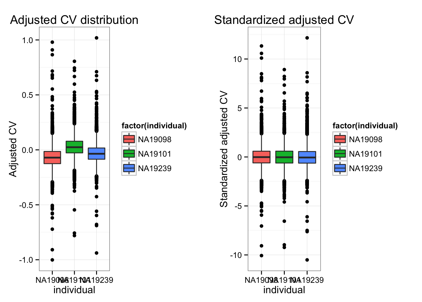
Compute metrics for quantifying similarity between the three individual coefficients of variation.
library(matrixStats)

df_norm <- as.data.frame(df_norm)
df_norm$squared_dev <- rowSums( ( df_norm - rowMedians(as.matrix(df_norm)) )^2 )
df_norm$abs_dev <- rowSums(abs( df_norm - rowMedians(as.matrix(df_norm)) ))
*Gene with the largest SSM (Sum-of-Squared-Deviation-from-the-median).
library(broman)
crayon <- brocolors("crayon")
library(scales)

gene <- rownames(molecules_ENSG)[ order(df_norm$squared_dev, decreasing = TRUE)[3]]

# Compute density for individual gene expression
dens <- lapply(1:3, function(ii_individual) {
   density( unlist(molecules_ENSG[ rownames(molecules_ENSG) == gene,
        anno_filter$individual == unique(anno_filter$individual)[ii_individual]]) )
  })
names(dens) <- unique(anno_filter$individual)
xlims <- c(range( sapply(dens, "[[", 1) ) )
ylims <- c(0, max( sapply(dens, "[[", 2) ) )

par(mfrow = c(1,1))
plot(0, pch = "",
     xlab = "log2 gene expression", main = "",
     ylab = "Density", axes = F, xlim = xlims, ylim = ylims)
axis(1); axis(2)
polygon(dens[[1]], col = alpha( crayon["Blue Bell"], .3), lwd = .5 )
polygon(dens[[2]], col = alpha( crayon["Fern"], .3), lwd = .5)
polygon(dens[[3]], col = alpha( crayon["Sunglow"], .2), lwd = .5 )
title(with(gene_info, external_gene_name[ensembl_gene_id == gene]) )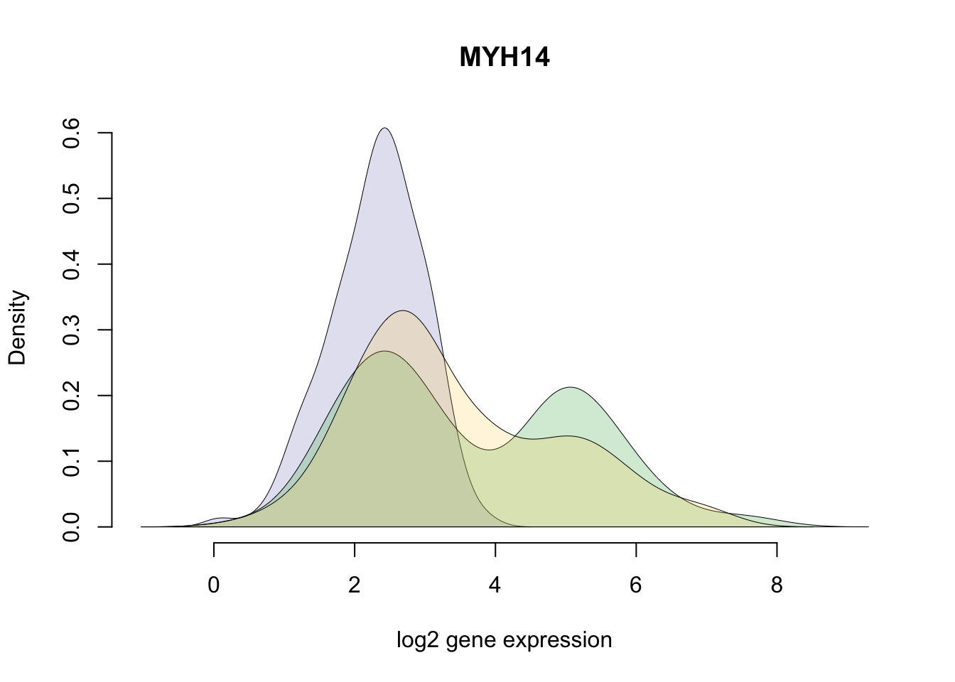
Session information
sessionInfo()R version 3.2.1 (2015-06-18)
Platform: x86_64-apple-darwin13.4.0 (64-bit)
Running under: OS X 10.10.5 (Yosemite)
locale:
[1] en_US.UTF-8/en_US.UTF-8/en_US.UTF-8/C/en_US.UTF-8/en_US.UTF-8
attached base packages:
[1] grid stats graphics grDevices utils datasets methods
[8] base
other attached packages:
[1] scales_0.3.0 broman_0.59-5 gridExtra_2.0.0
[4] matrixStats_0.15.0 zoo_1.7-12 Humanzee_0.1.0
[7] ggplot2_1.0.1 edgeR_3.10.5 limma_3.24.15
[10] dplyr_0.4.3 data.table_1.9.6 knitr_1.11
loaded via a namespace (and not attached):
[1] Rcpp_0.12.2 magrittr_1.5 MASS_7.3-45 munsell_0.4.2
[5] lattice_0.20-33 colorspace_1.2-6 R6_2.1.1 stringr_1.0.0
[9] plyr_1.8.3 tools_3.2.1 parallel_3.2.1 gtable_0.1.2
[13] DBI_0.3.1 htmltools_0.2.6 yaml_2.1.13 assertthat_0.1
[17] digest_0.6.8 reshape2_1.4.1 formatR_1.2.1 evaluate_0.8
[21] rmarkdown_0.8.1 labeling_0.3 stringi_1.0-1 chron_2.3-47
[25] proto_0.3-10