Cell-to-cell heterogeneity analysis summary
Joyce Hsiao
2015-11-17
- Objective
- Set up
- Prepare data
- Helper functions
- Cumulative distribution for ERCC spike-ins (filtered data)
- Individual CV-mean plot
- Compute normalized CV
- Venn diagram of top ranked genes
- GO analysis of top ranked genes
- Pluripotency and cell-cycle
- SSM (Sum of the Squared Deviation From the Median)
- GO analysis of differential CV genes
- Others
- Session information
Last updated: 2015-12-11
Code version: 7a25b2aef5c8329d4b5394cce595bbfc2b5b0c3e
Objective
In this document, I will outline and consolidate results of biological variation analysis.
Set up
library("data.table")
library("dplyr")
library("limma")
library("edgeR")
library("ggplot2")
library("grid")
theme_set(theme_bw(base_size = 12))
source("functions.R")
library("Humanzee")
library("cowplot")
Prepare data
Import annotation
Input annotation of only QC-filtered single cells. Remove NA19098.r2
anno_filter <- read.table("../data/annotation-filter.txt",
                      header = TRUE,
                      stringsAsFactors = FALSE)
dim(anno_filter)
[1] 568 5head(anno_filter, 2) individual replicate well batch sample_id
1 NA19098 r1 A01 NA19098.r1 NA19098.r1.A01
2 NA19098 r1 A02 NA19098.r1 NA19098.r1.A02Import molecule counts
Import molecule counts for genes with at least one observed read (before QC filtering).
molecules <- read.table("../data/molecules.txt",
                        header = TRUE, stringsAsFactors = FALSE)
dim(molecules)
[1] 18568 864molecules[1:5, 1:5] NA19098.r1.A01 NA19098.r1.A02 NA19098.r1.A03
ENSG00000186092 0 0 0
ENSG00000237683 1 0 3
ENSG00000185097 0 0 0
ENSG00000269831 0 0 0
ENSG00000188976 3 3 0
NA19098.r1.A04 NA19098.r1.A05
ENSG00000186092 0 0
ENSG00000237683 3 0
ENSG00000185097 0 0
ENSG00000269831 0 0
ENSG00000188976 2 7Remove genes with mean zero count in the unfiltered data
library(matrixStats)
molecules <- molecules[rowMeans(as.matrix(molecules)) > 0, ]
molecules <- molecules[rowVars(as.matrix(molecules)) > 0, ]
dim(molecules)
[1] 17771 864Import molecule counts after filtering and before any correction.
molecules_filter <- read.table("../data/molecules-filter.txt",
                               header = TRUE, stringsAsFactors = FALSE)
stopifnot(NROW(anno_filter) == NCOL(molecules_filter))
Compute collision correctecd counts.
molecules_collision <- -1024 * log(1 - molecules_filter / 1024)Import final processed molecule counts of endogeneous genes.
molecules_final <- read.table("../data/molecules-final.txt",
                             header = TRUE, stringsAsFactors = FALSE)
dim(molecules_final)
[1] 10564 568stopifnot(NROW(anno_filter) == NCOL(molecules_final))Import final processed molecule counts of ERCC genes.
molecules_cpm_ercc <- read.table("../data/molecules-cpm-ercc.txt",
                             header = TRUE, stringsAsFactors = FALSE)
dim(molecules_cpm_ercc)
[1] 34 568stopifnot(NROW(anno_filter) == NCOL(molecules_cpm_ercc))Import CPM corrected counts
molecules_cpm <- read.table("../data/molecules-cpm.txt",
                             header = TRUE, stringsAsFactors = FALSE)
dim(molecules_cpm)
[1] 10564 568stopifnot(NROW(anno_filter) == NCOL(molecules_cpm))Import gene symbols.
gene_symbols <- read.table(file = "../data/gene-info.txt", sep = "\t",
                           header = TRUE, stringsAsFactors = FALSE, quote = "")
Helper functions
Plot_poisson_cv
Plot for each individual CV versus mean. Mark ERCC genes.
Fit a poisson distribution based on the ERCC genes and overlay the fittedn line.
plot_poisson_cv <- function(molecules_ENSG, molecules_ERCC,
                            is_log2count = FALSE,
                            include_observed_ERCC = TRUE,
                            main){
    cbPalette <- c("#999999", "#0000FF", "#56B4E9", "#009E73",
                   "#F0E442", "#0072B2", "#D55E00", "#CC79A7")

    library(matrixStats)
    if (is_log2count == FALSE) {
        molecules_ENSG <- as.matrix(molecules_ENSG)
        molecules_ERCC <- as.matrix(molecules_ERCC)
    }
    if (is_log2count == TRUE) {
        molecules_ENSG <- 2^as.matrix(molecules_ENSG)
        molecules_ERCC <- 2^as.matrix(molecules_ERCC)
    }
    # defnine poisson function on a log x scale
    poisson.c <- function (x) {
        (10^x)^(0.5)/(10^x)
    }

    # compute the lossy factor based on ERCC
    ####   use LS: first define the function of f, then find the minimum
    ####   dont use the points from ERCC.mol.mean < 0.1 to fit.
    ercc_mean <- rowMeans(molecules_ERCC)
    ercc_cv   <- sqrt(rowVars(molecules_ERCC))/rowMeans(molecules_ERCC)

    # compute the sum of square errors
    target.fun <- function(f){
        sum( (ercc_cv[ercc_mean > 0.1] -
                sqrt( 1/( f*ercc_mean[ercc_mean>0.1]) ) )^2 )
    }
    # find out the minimum
    ans <- nlminb(0.05, target.fun, lower=0.0000001, upper=1)
    minipar <- ans$par
    # use the minimum to create the lossy poisson
    lossy.posson <- function (x) {
        1/sqrt((10^x)*minipar)
    }

    # 3 s.d.
    large_sd <- function (x) {
        3*(10^x)^(0.5)/(10^x)
    }

    if (include_observed_ERCC == TRUE) {
    return(
      ggplot(rbind(data.frame(means = rowMeans(molecules_ENSG),
                      cvs = sqrt(rowVars(molecules_ENSG))/rowMeans(molecules_ENSG),
                      gene_type = rep(1, NROW(molecules_ENSG))),
                 data.frame(means = ercc_mean,
                            cvs = ercc_cv,
                            gene_type = rep(2, NROW(molecules_ERCC)))),
           aes(x = means, y = cvs, col = as.factor(gene_type)) )  +
      geom_point(size = 2, alpha = 0.5) +
      stat_function(fun = large_sd, col= "#F0E442") +
      stat_function(fun = poisson.c, col= "#CC79A7")  +
      stat_function(fun = lossy.posson, col= "#56B4E9") +
      scale_x_log10() + scale_colour_manual(values = cbPalette) +
      labs(x = "log10 mean gene expression",
           y ="Coefficient of variation (CV)",
           title = main)
    )
    }
    if (include_observed_ERCC == FALSE) {
    return(
      ggplot(rbind(data.frame(means = rowMeans(molecules_ENSG),
                      cvs = sqrt(rowVars(molecules_ENSG))/rowMeans(molecules_ENSG),
                      gene_type = rep(1, NROW(molecules_ENSG))),
                 data.frame(means = ercc_mean,
                            cvs = ercc_cv,
                            gene_type = rep(2, NROW(molecules_ERCC)))),
           aes(x = means, y = cvs, col = as.factor(gene_type)) )  +
      geom_point(size = 2, alpha = 0.5) +
      stat_function(fun = large_sd, col= "#F0E442") +
      stat_function(fun = poisson.c, col= "#CC79A7")  +
      scale_x_log10() + scale_colour_manual(values = cbPalette) +
      labs(x = "log10 mean gene expression",
           y ="Coefficient of variation (CV)",
           title = main)
    )
    }
}
plot_density
Per gene density plots of large distances.
plot_density <- function(which_gene, labels, gene_symbols) {
  library(scales)
  library(broman)
  crayon <- brocolors("crayon")
  dens <- lapply(1:3, function(per_individual) {
     which_individual <-
       anno_filter$individual == unique(anno_filter$individual)[per_individual]
     density(unlist( molecules_ENSG[ genes == which_gene, which_individual] ) )
     })
  xlims <- range(sapply(dens, function(obj) obj$x))
  ylims <- range(sapply(dens, function(obj) obj$y))
  plot(dens[[1]],
       xlab = "log2 gene expression", main = "",
       ylab = "Density", axes = F, lwd = 0, xlim = xlims, ylim = ylims)
  polygon(dens[[1]], col = alpha(crayon["Sunset Orange"], .4), border = "grey40")
  polygon(dens[[2]], col = alpha(crayon["Tropical Rain Forest"], .6), border = "grey40")
  polygon(dens[[3]], col = alpha(crayon["Denim"], .3), border = "grey40")
  axis(1); axis(2)
  mtext(text = labels, side = 3)
  title(main = with(gene_symbols,
                external_gene_name[which(ensembl_gene_id == which_gene)]) )
}
Cumulative distribution for ERCC spike-ins (filtered data)
34 ERCC genes left after filtering.
NA19098
if(!file.exists("figure/cv-adjusted.Rmd/ercc-poission-NA19098.pdf")) {
  pdf(file = "figure/cv-adjusted.Rmd/ercc-poission-NA19098.pdf",
      width = 8, height = 10)
  molecules_filter_ercc <- molecules_filter[grep("ERCC", rownames(molecules_filter) ),
                                          grep("NA19098", colnames(molecules_filter) ) ]
  molecules_filter_ercc <- molecules_filter_ercc[order(rowMeans(molecules_filter_ercc),
                                                  decreasing = TRUE), ]
  ncells <- NCOL(molecules_filter_ercc)
  par(mfrow = c(4, 3), cex.main = 1,
      cex = .7, mar = c(3, 3, 3, 2))
  for (i in 1: NROW(molecules_filter_ercc)) {
      expression <- unlist(molecules_filter_ercc[i, ])
      expression <- expression[order(expression)]
      plot(x = expression,
           y = cumsum(expression)/max(cumsum(expression)),
           main = rownames(molecules_filter_ercc)[i])
      lines(ecdf(expression), col = "blue")
      x_seq <- seq(from = 0, to = max(expression),  by = 1)
      lines(x = x_seq,
            y = ppois(x_seq, mean(x_seq)),
            col = "red" )
  }
  dev.off()
}
NA19101
if(!file.exists("figure/cv-adjusted.Rmd/ercc-poission-NA19101.pdf")) {
  pdf(file = "figure/cv-adjusted.Rmd/ercc-poission-NA19101.pdf",
      width = 8, height = 10)
  molecules_filter_ercc <- molecules_filter[grep("ERCC", rownames(molecules_filter) ),
                                          grep("NA19101", colnames(molecules_filter) ) ]
  molecules_filter_ercc <- molecules_filter_ercc[order(rowMeans(molecules_filter_ercc),
                                                decreasing = TRUE), ]
  ncells <- NCOL(molecules_filter_ercc)
  par(mfrow = c(4, 3), cex.main = 1,
      cex = .7, mar = c(3, 3, 3, 2))
  for (i in 1: NROW(molecules_filter_ercc)) {
      expression <- unlist(molecules_filter_ercc[i, ])
      expression <- expression[order(expression)]
      plot(x = expression,
           y = cumsum(expression)/max(cumsum(expression)),
           main = rownames(molecules_filter_ercc)[i])
      lines(ecdf(expression), col = "blue")
      x_seq <- seq(from = 0, to = max(expression),  by = 1)
      lines(x = x_seq,
            y = ppois(x_seq, mean(x_seq)),
            col = "red" )
  }
  dev.off()
}
NA19239
if(!file.exists("figure/cv-adjusted.Rmd/ercc-poission-NA19239.pdf")) {
  pdf(file = "figure/cv-adjusted.Rmd/ercc-poission-NA19239.pdf",
      width = 8, height = 10)
  molecules_filter_ercc <- molecules_filter[grep("ERCC", rownames(molecules_filter) ),
                                          grep("NA19239", colnames(molecules_filter) ) ]
  molecules_filter_ercc <- molecules_filter_ercc[order(rowMeans(molecules_filter_ercc),
                                                decreasing = TRUE), ]
  ncells <- NCOL(molecules_filter_ercc)
  par(mfrow = c(4, 3), cex.main = 1,
      cex = .7, mar = c(3, 3, 3, 2))
  for (i in 1: NROW(molecules_filter_ercc)) {
      expression <- unlist(molecules_filter_ercc[i, ])
      expression <- expression[order(expression)]
      plot(x = expression,
           y = cumsum(expression)/max(cumsum(expression)),
           main = rownames(molecules_filter_ercc)[i])
      lines(ecdf(expression), col = "blue")
      x_seq <- seq(from = 0, to = max(expression),  by = 1)
      lines(x = x_seq,
            y = ppois(x_seq, mean(x_seq)),
            col = "red" )
  }
  dev.off()
}
Overall
if(!file.exists("figure/cv-adjusted.Rmd/ercc-poission-overall.pdf")) {
  pdf(file = "figure/cv-adjusted.Rmd/ercc-poission-overall.pdf",
      width = 8, height = 10)
  molecules_filter_ercc <- molecules_filter[grep("ERCC", rownames(molecules_filter) ), ]
  molecules_filter_ercc <- molecules_filter_ercc[order(rowMeans(molecules_filter_ercc),
                                                decreasing = TRUE), ]
  ncells <- NCOL(molecules_filter_ercc)
  par(mfrow = c(4, 3), cex.main = 1,
      cex = .7, mar = c(3, 3, 3, 2))
  for (i in 1: NROW(molecules_filter_ercc)) {
      expression <- unlist(molecules_filter_ercc[i, ])
      expression <- expression[order(expression)]
      plot(x = expression,
           y = cumsum(expression)/max(cumsum(expression)),
           main = rownames(molecules_filter_ercc)[i])
      lines(ecdf(expression), col = "blue")
      x_seq <- seq(from = 0, to = max(expression),  by = 1)
      lines(x = x_seq,
            y = ppois(x_seq, mean(x_seq)),
            col = "red" )
  }
  dev.off()
}
Individual CV-mean plot
Points marked blue are ERCC genes, based on the observed counts. Note that CPM correction for the endogeneous genes included only total molecule coutns of the endogeneous genes, and CPM correction for the ERCC genes included only total molecule counts of the ERCC genes. Because the total molecule counts of the endogeneous genes is about 100 times of the ERCC genes, the CPM corrected ERCC counts end up being 100 times of the CPM corrected endogeneous genes on average.
Blue line is the lossy Poission line predicted based on ERCC genes.
Pink/Purple line is based on Poisson distribution.
Yellow line describes a 3 times of the standard deviation of a Poisson distribution.
NA19098
theme_set(theme_bw(base_size = 8))
cowplot::plot_grid(
    plot_poisson_cv(molecules[ grep("ERCC", rownames(molecules), invert = TRUE),
                               grep("NA19098", colnames(molecules) ) ],
                    molecules[grep("ERCC", rownames(molecules) ),
                              grep("NA19098", colnames(molecules) ) ],
                    is_log2count = FALSE,
                    main = "Raw counts") +
                    theme(legend.position = "none"),
    plot_poisson_cv(molecules_filter[grep("ERCC", rownames(molecules_filter),
                                          invert = TRUE),
                                      anno_filter$individual == "NA19098"],
                    molecules_filter[grep("ERCC", rownames(molecules_filter)),
                                     anno_filter$individual == "NA19098"],
                    is_log2count = FALSE,
                    main = "Filtered counts") +
                    theme(legend.position = "none"),
    plot_poisson_cv(molecules_collision[grep("ERCC", rownames(molecules_filter),
                                      invert = TRUE),
                                  anno_filter$individual == "NA19098"],
                molecules_collision[grep("ERCC", rownames(molecules_filter)),
                                 anno_filter$individual == "NA19098"],
                is_log2count = FALSE,
                main = "Collision-corrected counts") +
                theme(legend.position = "none"),
    plot_poisson_cv(molecules_filter[grep("ERCC", rownames(molecules_filter),
                                      invert = TRUE),
                                  anno_filter$individual == "NA19098"],
                molecules_filter[grep("ERCC", rownames(molecules_filter)),
                                 anno_filter$individual == "NA19098"],
                is_log2count = FALSE,
                main = "Filtered counts (zoom-in)") +
                theme(legend.position = "none") +
                ylim(0, 3),
  ncol = 2,
  labels = LETTERS[1:3])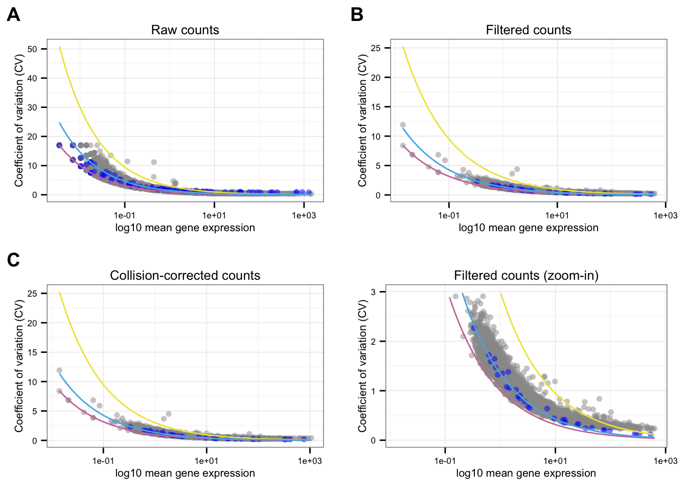
*NA19101
theme_set(theme_bw(base_size = 8))
cowplot::plot_grid(
    plot_poisson_cv(molecules[ grep("ERCC", rownames(molecules), invert = TRUE),
                               grep("NA19101", colnames(molecules) ) ],
                    molecules[grep("ERCC", rownames(molecules) ),
                              grep("NA19101", colnames(molecules) ) ],
                    is_log2count = FALSE,
                    main = "Raw counts") +
                    theme(legend.position = "none"),
    plot_poisson_cv(molecules_filter[grep("ERCC", rownames(molecules_filter),
                                          invert = TRUE),
                                      anno_filter$individual == "NA19101"],
                    molecules_filter[grep("ERCC", rownames(molecules_filter)),
                                     anno_filter$individual == "NA19101"],
                    is_log2count = FALSE,
                    main = "Filtered counts") +
                    theme(legend.position = "none"),
    plot_poisson_cv(molecules_collision[grep("ERCC", rownames(molecules_filter),
                                      invert = TRUE),
                                  anno_filter$individual == "NA19101"],
                molecules_collision[grep("ERCC", rownames(molecules_filter)),
                                 anno_filter$individual == "NA19101"],
                is_log2count = FALSE,
                main = "Collision-corrected counts") +
                theme(legend.position = "none"),
    plot_poisson_cv(molecules_filter[grep("ERCC", rownames(molecules_filter),
                                          invert = TRUE),
                                      anno_filter$individual == "NA19101"],
                    molecules_filter[grep("ERCC", rownames(molecules_filter)),
                                     anno_filter$individual == "NA19101"],
                    is_log2count = FALSE,
                    main = "Filtered counts (zoom-in)") +
                    theme(legend.position = "none") +
                    ylim(0, 3),
    ncol = 2,
    labels = LETTERS[1:4])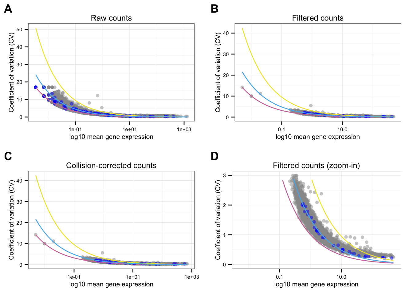
*NA19239
theme_set(theme_bw(base_size = 8))
cowplot::plot_grid(
    plot_poisson_cv(molecules[ grep("ERCC", rownames(molecules), invert = TRUE),
                               grep("NA19239", colnames(molecules) ) ],
                    molecules[grep("ERCC", rownames(molecules) ),
                              grep("NA19239", colnames(molecules) ) ],
                    is_log2count = FALSE,
                    main = "Raw counts") +
                    theme(legend.position = "none"),
    plot_poisson_cv(molecules_filter[grep("ERCC", rownames(molecules_filter),
                                          invert = TRUE),
                                      anno_filter$individual == "NA19239"],
                    molecules_filter[grep("ERCC", rownames(molecules_filter)),
                                     anno_filter$individual == "NA19239"],
                    is_log2count = FALSE,
                    main = "Filtered counts") +
                    theme(legend.position = "none"),
    plot_poisson_cv(molecules_collision[grep("ERCC", rownames(molecules_filter),
                                      invert = TRUE),
                                  anno_filter$individual == "NA19239"],
                molecules_collision[grep("ERCC", rownames(molecules_filter)),
                                 anno_filter$individual == "NA19239"],
                is_log2count = FALSE,
                main = "Collision-corrected counts") +
                theme(legend.position = "none"),
    plot_poisson_cv(molecules_filter[grep("ERCC", rownames(molecules_filter),
                                          invert = TRUE),
                                      anno_filter$individual == "NA19239"],
                    molecules_filter[grep("ERCC", rownames(molecules_filter)),
                                     anno_filter$individual == "NA19239"],
                    is_log2count = FALSE,
                    main = "Filtered counts (zoom-in)") +
                    theme(legend.position = "none") +
                    ylim(0, 3),
    ncol = 2,
  labels = LETTERS[1:4])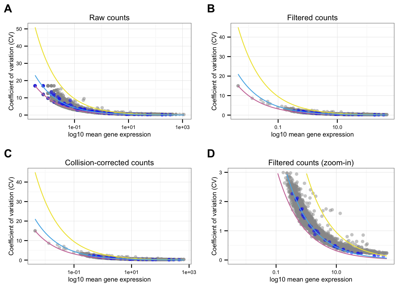
Compute normalized CV
- Compute Squared Coefficients of Variation across cells for each individual;
- Adjust Squared CVs for confounding effect with the mean:
- Compute rolling medians of gene expression levels,
- Compute Squared CVs corresponding to rolling medians of gene expression levels,
- Standardize the adjusted Squared CV across each individual’s mean and standard deviation of adjusted CVs.
Load functions to compute and to adjust CVs.
source("../code/cv-functions.r")Compute individual CVs.
ENSG_cv <- compute_cv(log2counts = molecules_final,
                      grouping_vector = anno_filter$individual)
Adjust CVs for mean dependency.
ENSG_cv_adj <- normalize_cv(group_cv = ENSG_cv,
                            log2counts = molecules_final,
                            anno = anno_filter)
Standardized CVs.
df_cv <- data.frame(NA19098 = ENSG_cv_adj[[1]]$log10cv2_adj,
                    NA19101 = ENSG_cv_adj[[2]]$log10cv2_adj,
                    NA19239 = ENSG_cv_adj[[3]]$log10cv2_adj)

library(matrixStats)
df_norm <- sweep(df_cv, MARGIN = 2, STATS = colMeans(as.matrix(df_cv)), FUN = "-")
df_norm <- sweep(df_norm, MARGIN = 2, STATS = sqrt(colVars(as.matrix(df_cv))), FUN = "/")
CV before versus after adjustement.
theme_set(theme_bw(base_size = 8))
plot_grid(
  ggplot(data.frame(means = c(ENSG_cv[[1]]$mean, ENSG_cv[[2]]$mean, ENSG_cv[[3]]$mean),
                  individual = rep( names(ENSG_cv), each = NROW(ENSG_cv[[1]]) ) ),
         aes(x = factor(individual), y = log10(means), fill = individual ) ) +
      geom_violin(alpha = .6) + geom_boxplot(alpha = .2, width = .2) +
      xlab("Individual") + ylab("Mean gene expression level") +
      ggtitle("Global gene expression profile") + theme(legend.position = "none"),
  ggplot(data.frame(cv = c(ENSG_cv[[1]]$cv, ENSG_cv[[2]]$cv, ENSG_cv[[3]]$cv),
                  individual = rep( names(ENSG_cv), each = NROW(ENSG_cv[[1]]) ) ),
         aes(x = factor(individual), y = log10(cv^2), fill = individual ) ) +
      geom_violin(alpha = .6) + geom_boxplot(alpha = .2, width = .2) +
      xlab("Individual") + ylab("log10 CV^2") +
      ggtitle("Global noise measure by Squared CV") +
      theme(legend.position = "none"),
  ggplot(data.frame(cv = c(ENSG_cv_adj[[1]]$log10cv2_adj,
                           ENSG_cv_adj[[2]]$log10cv2_adj,
                           ENSG_cv_adj[[3]]$log10cv2_adj),
                    individual = rep( names(ENSG_cv), each = NROW(ENSG_cv[[1]]) ) ),
         aes(x = factor(individual), y = cv, fill = individual ) ) +
      geom_violin(alpha = .6) + geom_boxplot(alpha = .2, width = .2) +
      xlab("Individual") + ylab("Adjusted log10 CV^2") +
      ggtitle("Global mean-adjusted noise measure") +
      theme(legend.position = "none"),
  ggplot(data.frame(cv = c(df_norm$NA19098,
                           df_norm$NA19101,
                           df_norm$NA19239),
                    individual = rep( names(ENSG_cv), each = NROW(ENSG_cv[[1]]) ) ),
         aes(x = factor(individual), y = cv, fill = individual ) ) +
      geom_violin(alpha = .6) + geom_boxplot(alpha = .2, width = .2) +
      xlab("Individual") + ylab("Standardized adjusted log10 CV^2") +
      ggtitle("SCV") + theme(legend.position = "none"),
  labels = LETTERS[1:4] )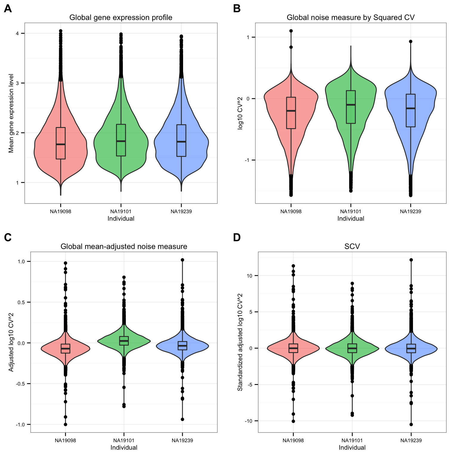
CV versus mean plot
theme_set(theme_bw(base_size = 8))
plot_grid(
  ggplot(data.frame(means = c(ENSG_cv[[1]]$mean, ENSG_cv[[2]]$mean, ENSG_cv[[3]]$mean),
                    cvs = c(ENSG_cv[[1]]$cv, ENSG_cv[[2]]$cv, ENSG_cv[[3]]$cv),
                  individual = rep( names(ENSG_cv), each = NROW(ENSG_cv[[1]]) ) ),
         aes(x = log10(means), y = log10(cvs) ) ) +
      geom_point( aes( colour = factor(individual) ), size = .9)  +
      xlab("log10 Mean gene expression level") + ylab("log10 Squared CV") +
      theme(legend.position = "none"),
  ggplot(data.frame(means = c(ENSG_cv[[1]]$mean, ENSG_cv[[2]]$mean, ENSG_cv[[3]]$mean),
                    cvs = c(df_norm$NA19098, df_norm$NA19101, df_norm$NA19239),
                  individual = rep( names(ENSG_cv), each = NROW(ENSG_cv[[1]]) ) ),
         aes(x = log10(means), y = cvs) ) +
      geom_point( aes( colour = factor(individual) ),
                  size = 1.2, alpha = .8)  +
      xlab("log10 Mean gene expression level") + ylab("SCV (Standardized CV)") +
      theme(legend.position = "none"),
  ggplot(data.frame(NA19098 = log10(ENSG_cv[[1]]$mean),
                  NA19101 = log10(ENSG_cv[[2]]$mean) ),
       aes(x = NA19098, y = NA19101 ) ) +
    geom_point(size = 1.2) + xlim(.7, 4.3) + ylim(.7, 4.3) +
    xlab("NA19098") + ylab("NA19101") + geom_abline(slope = 1, col = "darkblue") +
    ggtitle("Individual log10 mean gene expression levels") +
    theme(legend.position = "none"),
  ggplot(data.frame(NA19098 = log10(ENSG_cv[[1]]$cv^2),
                    NA19101 = log10(ENSG_cv[[2]]$cv^2) ),
         aes(x = NA19098, y = NA19101 ) ) +
      geom_point(size = 1.2) + xlim(-2, 1.5) + ylim(-2, 1.5) +
      xlab("NA19098") + ylab("NA19101") + geom_abline(slope = 1, col = "darkblue") +
      ggtitle("Individual noise measure by Squared CV") +
      theme(legend.position = "none"),
  ggplot(data.frame( NA19098 = df_norm$NA19098,
                     NA19101 = df_norm$NA19101 ),
         aes(x = NA19098, y = NA19101 ) ) +
      geom_point(size = 1.2) + xlim(-11, 11.5) + ylim(-11, 11.5) +
      xlab("NA19098") + ylab("NA19101") + geom_abline(slope = 1, col = "darkblue") +
      ggtitle("Individual SCV measure") +
      theme(legend.position = "none"),
  ncol = 2, nrow = 3,
  labels = LETTERS[1:5] )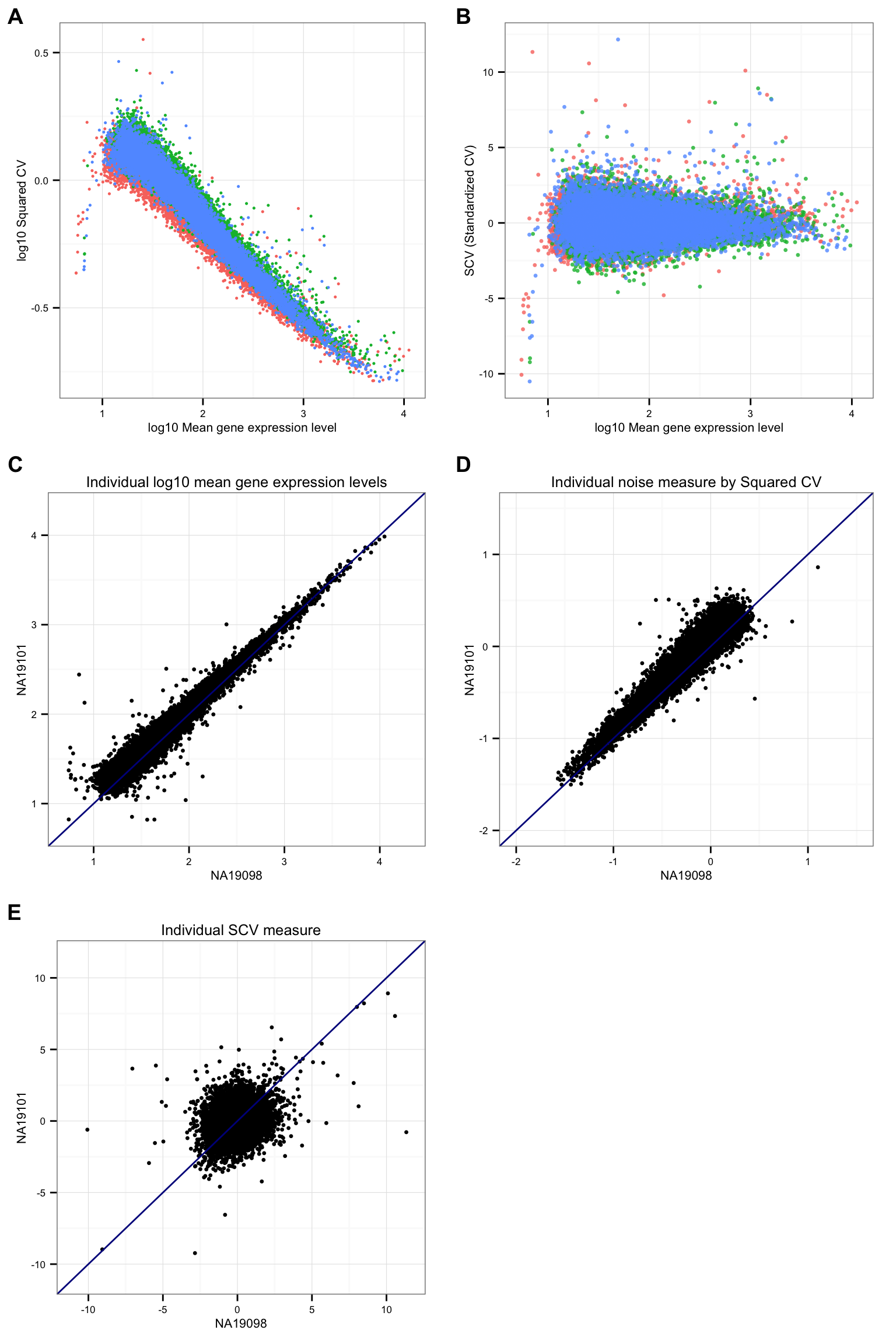
Venn diagram of top ranked genes
Top 1000 genes based on Standardized CVs.
genes <- rownames(ENSG_cv[[1]])
library(gplots)
gplots::venn(
  list(NA19098 = genes[ which( rank(df_norm[[1]]) > length(genes) - 1000 ) ],
       NA19101 = genes[ which( rank(df_norm[[2]]) > length(genes) - 1000 ) ],
       NA19239 = genes[ which( rank(df_norm[[3]]) > length(genes) - 1000 ) ] ))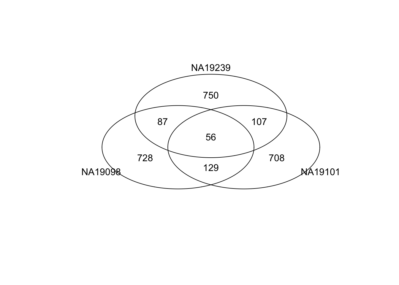
Top 1000 genes based on Means.
genes <- rownames(ENSG_cv[[1]])
library(gplots)
gplots::venn(
  list(NA19098 = genes[ which(rank(ENSG_cv[[1]]$mean) > length(genes) - 1000 ) ],
       NA19101 = genes[ which(rank(ENSG_cv[[2]]$mean) > length(genes) - 1000 ) ],
       NA19239 = genes[ which(rank(ENSG_cv[[3]]$mean) > length(genes) - 1000 ) ] ) )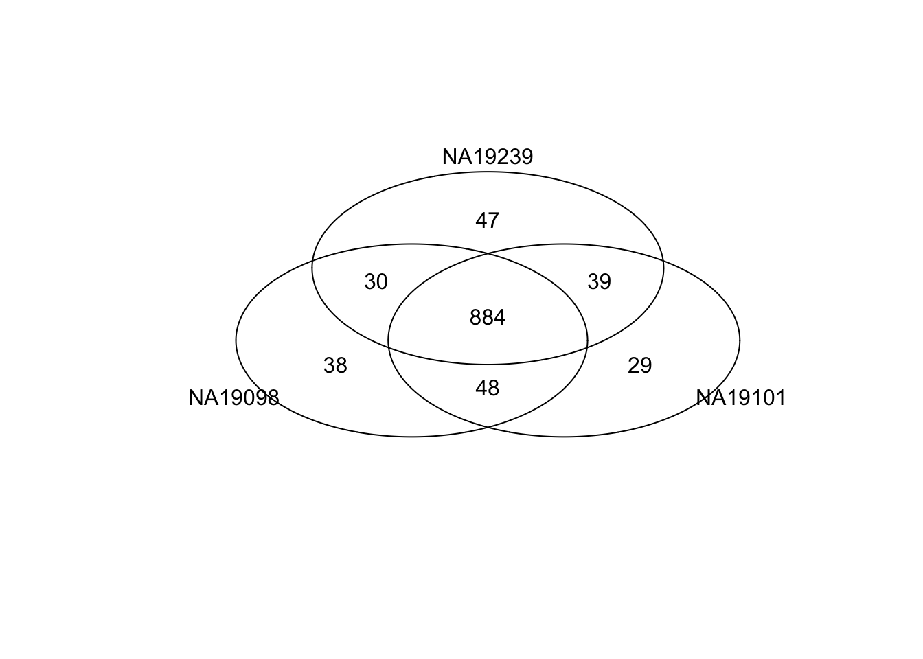
Mark top ranked genes based on individual standardized CVs.
df_plot <- data.frame(
  cvs = c(ENSG_cv_adj[[1]]$log10cv2_adj, ENSG_cv_adj[[2]]$log10cv2_adj,
          ENSG_cv_adj[[3]]$log10cv2_adj),
  normed_cv = c(df_norm$NA19098, df_norm$NA19101, df_norm$NA19239),
  means = c(ENSG_cv[[1]]$mean, ENSG_cv[[2]]$mean, ENSG_cv[[3]]$mean),
  individual = as.factor(rep(names(ENSG_cv), each = NROW(ENSG_cv[[1]])) ) )

cowplot::plot_grid(
  ggplot( df_plot,
      aes(x = log10(means), y = normed_cv ) ) +
      geom_point( aes(col = as.factor(individual)), cex = 1.2 ) +
      facet_wrap( ~ individual) +
      labs(x = "log10 Mean gene expression level",
           y = "Standardized CV") +
      geom_point(
        data = df_plot[ rep( rank(ENSG_cv[[1]]$mean) > length(genes) - 1000, 3), ],
        colour = "grey20", cex = 1.2 ) +
      ggtitle("Top 1000 genes by NA19098 mean gene expressionl ") +
      theme(legend.position = "none"),
  ggplot( df_plot,
        aes(x = log10(means), y = normed_cv ) ) +
        geom_point( aes(col = as.factor(individual)), cex = 1.2 ) +
        facet_wrap( ~ individual) +
        labs(x = "log10 Mean gene expression level",
             y = "Standardized CV") +
        geom_point(
          data = df_plot[ rep( rank(df_norm[[1]]) > length(genes) - 1000, 3), ],
          colour = "grey20", cex = 1.2 ) +
        ggtitle("Top 1000 genes by NA19098 SCV") +
        theme(legend.position = "none"),
  ggplot( df_plot,
        aes(x = log10(means), y = normed_cv ) ) +
        geom_point( aes(col = as.factor(individual)), cex = 1.2 ) +
        facet_wrap( ~ individual) +
        labs(x = "log10 Mean gene expression level",
             y = "Standadrdized CV") +
        geom_point(
          data = df_plot[ rep( rank(df_norm[[2]]) > length(genes) - 1000, 3), ],
          colour = "grey20", cex = .9 ) +
        ggtitle("Top 1000 genes by NA19101 SCV") +
        theme(legend.position = "none"),
  ggplot( df_plot,
        aes(x = log10(means), y = normed_cv ) ) +
        geom_point( aes(col = as.factor(individual)), cex = 1.2 ) +
        facet_wrap( ~ individual) +
        labs(x = "log10 Mean gene expression level",
             y = "log10 Squared CV") +
        geom_point(
          data = df_plot[ rep( rank(df_norm[[3]]) > length(genes) - 1000, 3), ],
          colour = "grey20", cex = 1.2 ) +
        ggtitle("Top 1000 genes by NA19239 SCV") +
        theme(legend.position = "none"),
labels = LETTERS[1:4] ) 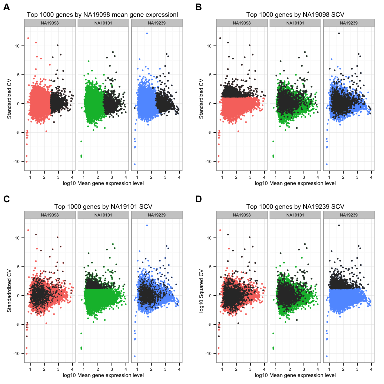
GO analysis of top ranked genes
Based on Standardized CVs
if (!file.exists("rda/cv-adjusted-summary/go-cv-rank.rda")) {
  venn_cv_rank <- gplots::venn(
      list(NA19098 = genes[ which( rank(df_norm[[1]]) > length(genes) - 1000 ) ],
           NA19101 = genes[ which( rank(df_norm[[2]]) > length(genes) - 1000 ) ],
           NA19239 = genes[ which( rank(df_norm[[3]]) > length(genes) - 1000 ) ] ))
  venn_cv_rank_list <- attr(venn_cv_rank, "intersections")

  # GO terms of genes with high CV across individuals
  go_cv_rank_all <- GOtest(my_ensembl_gene_universe = rownames(molecules_filter),
                            my_ensembl_gene_test = venn_cv_rank_list[["111"]],
                            pval_cutoff = 1, ontology=c("BP") )
  go_cv_rank_all_terms <- summary(go_cv_rank_all$GO$BP, pvalue = 1)
  go_cv_rank_all_terms <- data.frame(ID = go_cv_rank_all_terms[[1]],
                                     Pvalue = go_cv_rank_all_terms[[2]],
                                     Terms = go_cv_rank_all_terms[[7]])
  go_cv_rank_all_terms <- go_cv_rank_all_terms[order(go_cv_rank_all_terms$Pvalue), ]

  # GO terms of genes with high CVs for NA19098
  go_cv_rank_NA19098 <- GOtest(my_ensembl_gene_universe = rownames(molecules_filter),
                            my_ensembl_gene_test = venn_cv_rank_list[["100"]],
                            pval_cutoff = 1, ontology=c("BP") )
  go_cv_rank_NA19098_terms <- summary(go_cv_rank_NA19098$GO$BP, pvalue = 1)
  go_cv_rank_NA19098_terms <- data.frame(ID = go_cv_rank_NA19098_terms[[1]],
                                     Pvalue = go_cv_rank_NA19098_terms[[2]],
                                     Terms = go_cv_rank_NA19098_terms[[7]])
  go_cv_rank_NA19098_terms <- go_cv_rank_NA19098_terms[order(go_cv_rank_NA19098_terms$Pvalue), ]

  # GO terms of genes with high CVs for NA19101
  go_cv_rank_NA19101 <- GOtest(my_ensembl_gene_universe = rownames(molecules_filter),
                            my_ensembl_gene_test = venn_cv_rank_list[["010"]],
                            pval_cutoff = 1, ontology=c("BP") )
  go_cv_rank_NA19101_terms <- summary(go_cv_rank_NA19101$GO$BP, pvalue = 1)
  go_cv_rank_NA19101_terms <- data.frame(ID = go_cv_rank_NA19101_terms[[1]],
                                     Pvalue = go_cv_rank_NA19101_terms[[2]],
                                     Terms = go_cv_rank_NA19101_terms[[7]])
  go_cv_rank_NA19101_terms <- go_cv_rank_NA19101_terms[order(go_cv_rank_NA19101_terms$Pvalue), ]


  # GO terms of genes with high CVs for NA19239
  go_cv_rank_NA19239 <- GOtest(my_ensembl_gene_universe = rownames(molecules_filter),
                            my_ensembl_gene_test = venn_cv_rank_list[["001"]],
                            pval_cutoff = 1, ontology=c("BP") )
  go_cv_rank_NA19239_terms <- summary(go_cv_rank_NA19239$GO$BP, pvalue = 1)
  go_cv_rank_NA19239_terms <- data.frame(ID = go_cv_rank_NA19239_terms[[1]],
                                     Pvalue = go_cv_rank_NA19239_terms[[2]],
                                     Terms = go_cv_rank_NA19239_terms[[7]])
  go_cv_rank_NA19239_terms <- go_cv_rank_NA19239_terms[order(go_cv_rank_NA19239_terms$Pvalue), ]

  save(go_cv_rank_all_terms,
       go_cv_rank_NA19098_terms, go_cv_rank_NA19101_terms, go_cv_rank_NA19239_terms,
       file = "rda/cv-adjusted-summary/go-cv-rank.rda")
} else {
  load(file = "rda/cv-adjusted-summary/go-cv-rank.rda")
}
Pluripotency and cell-cycle
Import cell-cycle gene list.
cellcycle_genes <- read.table("../data/cellcyclegenes.txt", sep = "\t",
                              header = TRUE, stringsAsFactors = FALSE)
str(cellcycle_genes)
'data.frame': 151 obs. of 5 variables:
$ G1.S: chr "ENSG00000102977" "ENSG00000119640" "ENSG00000154734" "ENSG00000088448" ...
$ S : chr "ENSG00000114770" "ENSG00000144827" "ENSG00000180071" "ENSG00000105011" ...
$ G2.M: chr "ENSG00000011426" "ENSG00000065000" "ENSG00000213390" "ENSG00000122644" ...
$ M : chr "ENSG00000135541" "ENSG00000135334" "ENSG00000154945" "ENSG00000011426" ...
$ M.G1: chr "ENSG00000173744" "ENSG00000160216" "ENSG00000170776" "ENSG00000218624" ...Mark cell-cycle genes.
ii_cellcycle_genes <- lapply(1:3, function(per_individual) {
  genes %in% unlist(cellcycle_genes)
})
names(ii_cellcycle_genes) <- names(ENSG_cv)
ii_cellcycle_genes <- do.call(c, ii_cellcycle_genes)

ggplot(data.frame(do.call(rbind, ENSG_cv_adj),
                  normed_cv = c(df_norm$NA19098, df_norm$NA19101, df_norm$NA19239) ),
       aes(x = log10(mean), y = normed_cv )) +
  geom_point(aes(col = group), cex = 1.2) + facet_wrap( ~ group) +
  ggtitle("Cellcycle genes") +
  geom_point(
      data = subset(data.frame(do.call(rbind, ENSG_cv_adj),
                 normed_cv = c(df_norm$NA19098, df_norm$NA19101, df_norm$NA19239) ),
                 ii_cellcycle_genes),
       colour = "grey20", cex = 1.2) +
  labs(x = "log10 Mean gene expression level",
       y = "Standardized CV")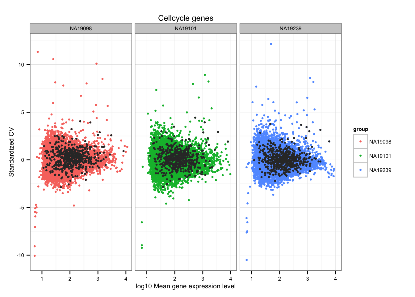
Import pluripotent gene list
pluripotent_genes <- read.table("../data/pluripotency-genes.txt", sep = "\t",
                              header = TRUE, stringsAsFactors = FALSE)
str(pluripotent_genes)
'data.frame': 27 obs. of 4 variables:
$ From : chr "GDF3" "ZFP42" "NR6A1" "SOX2" ...
$ To : chr "ENSG00000184344" "ENSG00000179059" "ENSG00000148200" "ENSG00000181449" ...
$ Species : chr "Homo sapiens" "Homo sapiens" "Homo sapiens" "Homo sapiens" ...
$ Gene.Name: chr "growth differentiation factor 3" "zinc finger protein 42 homolog (mouse)" "nuclear receptor subfamily 6, group A, member 1" "SRY (sex determining region Y)-box 2" ...Mark pluripotent genes
ii_pluripotent_genes <- lapply(1:3, function(per_individual) {
  genes %in% unlist(pluripotent_genes$To)
})
names(ii_pluripotent_genes) <- names(ENSG_cv)
ii_pluripotent_genes <- do.call(c, ii_pluripotent_genes)

ggplot(data.frame(do.call(rbind, ENSG_cv_adj),
                  normed_cv = c(df_norm$NA19098, df_norm$NA19101, df_norm$NA19239) ),
       aes(x = log10(mean), y = normed_cv)) +
  geom_point(aes(col = group), cex = 1.2) + facet_wrap( ~ group) +
  ggtitle("Pluripotent genes") +
  geom_point(data = subset(data.frame(do.call(rbind, ENSG_cv_adj),
                  normed_cv = c(df_norm$NA19098, df_norm$NA19101, df_norm$NA19239) ),
                           ii_pluripotent_genes),
             colour = "grey20", cex = 1.2) +
  labs(x = "log10 Mean gene expression level",
       y = "log10 SCV")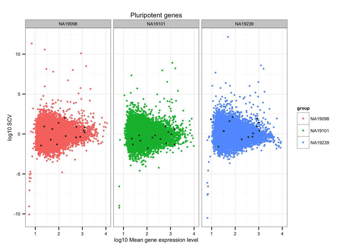
SSM (Sum of the Squared Deviation From the Median)
Compute SSM.
library(matrixStats)
df_norm$squared_dev <- rowSums( ( df_norm - rowMedians(as.matrix(df_norm)) )^2 )
Top 1000 ranked genes by SSM.
ggplot(data.frame(do.call(rbind, ENSG_cv_adj),
                  normed_cv = c(df_norm$NA19098, df_norm$NA19101, df_norm$NA19239) ),
       aes(x = log10(mean), y = normed_cv )) +
  geom_point(aes(col = group), cex = 1.2) + facet_wrap( ~ group) +
  ggtitle("Top 1000 ranked genes by SSM") +
  geom_point(
    data = subset(data.frame(do.call(rbind, ENSG_cv_adj),
                  normed_cv = c(df_norm$NA19098, df_norm$NA19101, df_norm$NA19239) ),
                  rep(rank(df_norm$squared_dev) > length(genes) - 1000, times = 3) ),
             colour = "grey20", cex = 1.2 ) +
  labs(x = "log10 Mean gene expression level",
       y = "SCV")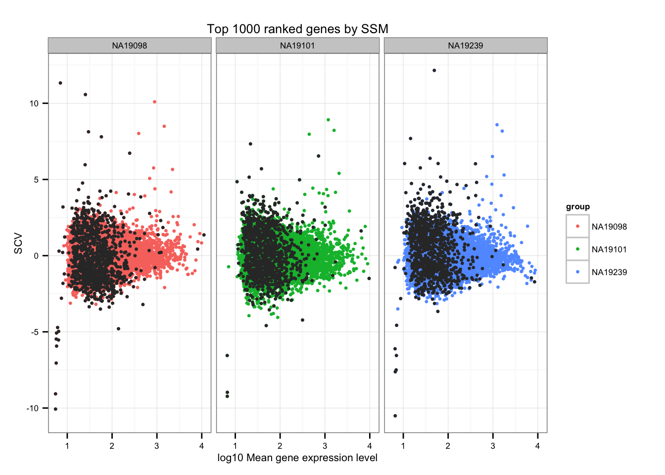
Import permutation results.
load("rda/cv-adjusted-statistical-test-permute/permuted-pval.rda")
sum(permuted_pval$squared_dev == 0)
[1] 96Histogram
ggplot( data.frame(pvals = permuted_pval$squared_dev),
       aes(x = pvals) ) +
  geom_histogram() + xlim(0, 1) +
  labs(x = "Permutation-based p-values", y = "Count")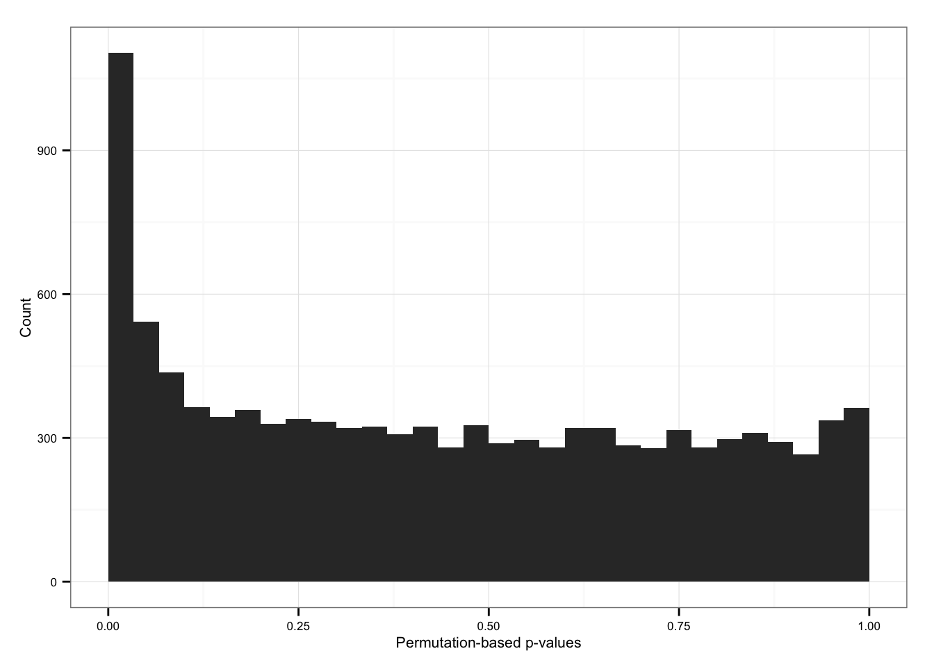
P-value versus distance
ggplot( data.frame(pvals = permuted_pval$squared_dev,
                   dist = df_norm$squared_dev),
        aes( x = dist, y = pvals)) +
geom_point(size = 1.2) 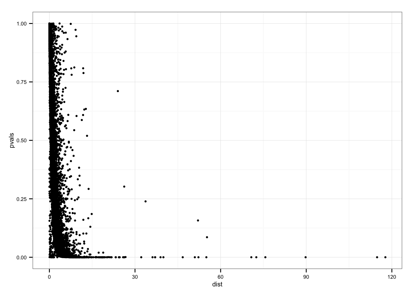
summary(df_norm$squared_dev[permuted_pval$squared_dev == 0]) Min. 1st Qu. Median Mean 3rd Qu. Max.
0.6657 10.4900 14.1900 21.3700 22.1600 117.7000 Genes with p = 0 sorted by SSM
if(!file.exists("../analysis/figure/cv-adjusted-summary.Rmd/density-high-ssm.pdf")) {
    pdf(file = "../analysis/figure/cv-adjusted-summary.Rmd/density-high-ssm.pdf",
        height = 12, width = 8)
    genes_plot <- data.frame(pval = permuted_pval$squared_dev,
                             dist = df_norm$squared_dev,
                             genes = genes)
    genes_plot <- genes_plot[ order(genes_plot$dist, decreasing = TRUE), ]
    genes_plot <- genes_plot[ genes_plot$pval == 0, ]
    par(mfrow = c(5,4), cex = .7)
    for(i in 1:dim(genes_plot)[1]) {
      plot_density(genes_plot$genes[i],
                   labels = round(genes_plot$dist[i], 6),
                   gene_symbols = gene_symbols)
    }
    dev.off()
}
Genes with non-significant SSM
if(!file.exists("../analysis/figure/cv-adjusted-summary.Rmd/density-low-ssm.pdf")) {
    pdf(file = "../analysis/figure/cv-adjusted-summary.Rmd/density-low-ssm.pdf",
        height = 12, width = 8)
    genes_plot <- data.frame(pval = permuted_pval$squared_dev,
                             dist = df_norm$squared_dev,
                             genes = genes)
    genes_plot <- genes_plot[ order(genes_plot$dist,
                                    genes_plot$pval, decreasing = FALSE), ]
    par(mfrow = c(5,4), cex = .7)
    for(i in 1:60) {
      plot_density(genes_plot$genes[i],
                   labels = round(genes_plot$dist[i], 6),
                   gene_symbols = gene_symbols)
    }
    dev.off()
}
GO analysis of differential CV genes
if (!file.exists("rda/cv-adjusted-summary/go.rda")) {
  go_cv <- GOtest(my_ensembl_gene_universe = rownames(molecules_filter),
                      my_ensembl_gene_test = rownames(molecules_filter)[permuted_pval$squared_dev == 0],
                      pval_cutoff = 1, ontology=c("BP") )
  goterms_bp <- summary(go_cv$GO$BP, pvalue = 1)
  goterms_bp <- data.frame(ID = goterms_bp[[1]],
                           Pvalue = goterms_bp[[2]],
                           Terms = goterms_bp[[7]])
  goterms_bp <- goterms_bp[order(goterms_bp$Pvalue), ]
} else {
  load(file = "rda/cv-adjusted-summary/go.rda")
}
goterms_bp$Terms[ goterms_bp$Pvalue < .01 ]
[1] cellular response to zinc ion
[2] cellular response to cadmium ion
[3] cell-cell adhesion via plasma-membrane adhesion molecules
[4] cell-cell adhesion
[5] response to zinc ion
[6] response to cadmium ion
[7] calcium-independent cell-cell adhesion via plasma membrane cell-adhesion molecules
[8] response to interferon-beta
[9] mitotic cell cycle arrest
[10] response to interferon-alpha
[11] negative regulation of growth
[12] homophilic cell adhesion via plasma membrane adhesion molecules
[13] skeletal muscle contraction
[14] cleavage in ITS2 between 5.8S rRNA and LSU-rRNA of tricistronic rRNA transcript (SSU-rRNA, 5.8S rRNA, LSU-rRNA)
[15] chitin metabolic process
[16] chitin catabolic process
[17] blood coagulation, extrinsic pathway
[18] positive regulation of skeletal muscle contraction by regulation of release of sequestered calcium ion
[19] phosphatidylinositol catabolic process
[20] actin phosphorylation
[21] regulation of actin phosphorylation
[22] regulation of integrin biosynthetic process
[23] negative regulation of integrin biosynthetic process
[24] positive regulation of integrin biosynthetic process
[25] pattern specification involved in kidney development
[26] nuclear polyadenylation-dependent mRNA catabolic process
[27] polyadenylation-dependent mRNA catabolic process
[28] proximal/distal pattern formation involved in nephron development
[29] renal system pattern specification
[30] specification of nephron tubule identity
[31] specification of loop of Henle identity
[32] pattern specification involved in metanephros development
[33] proximal/distal pattern formation involved in metanephric nephron development
[34] mitochondrial mRNA processing
[35] mitochondrial mRNA 3'-end processing
[36] mitochondrial mRNA polyadenylation
[37] negative regulation of cytokine production involved in inflammatory response
[38] negative regulation of sperm motility
[39] protein K33-linked ubiquitination
[40] regulation of miRNA catabolic process
[41] positive regulation of miRNA catabolic process
1681 Levels: actin cytoskeleton organization ... zymogen activationOthers
Sparsity
- High SSM genes.
Make a data.frame for all genes tested including permutation-based p-values, SSM (Sum-of-the-Squared-Deviations-From-the-Median), ENSG IDs, and gene symbols.
genes_plot <- data.frame(
    pval = permuted_pval$squared_dev,
    dist = df_norm$squared_dev,
    genes = genes,
    gene_symbols = with(gene_symbols,
                        external_gene_name[match(genes, ensembl_gene_id)]) )
genes_plot <- genes_plot[ order(genes_plot$dist, decreasing = TRUE), ]
genes_plot <- genes_plot[ genes_plot$pval == 0, ]
For each individual, count the number of zero count cells and the number of non-zero count cells.
library(gridExtra)
grid.arrange(grobs = lapply(1:16, function(per_gene) {
  zero_count <- molecules_filter[rownames(molecules_filter) == genes_plot$genes[per_gene], ] == 0
  ggplot(data.frame(zero_count = c(zero_count),
                    individual = anno_filter$individual),
         aes(x = factor(individual),
             fill = zero_count,
             color = individual) ) +
         geom_bar() + scale_fill_grey() +
         ggtitle(genes_plot$gene_symbols[per_gene]) +
         theme(legend.position = "none")
  }),
  ncol = 4, nrow = 4,
  labels = LETTERS[1:16])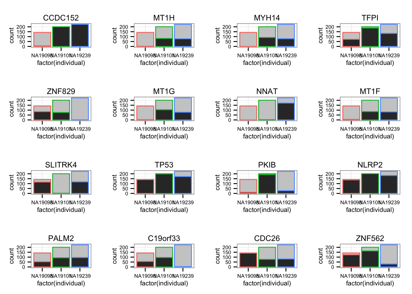
Heatmap
Placeholder for a heatmap.
library(gplots)
library(broman)
crayon <- brocolors("crayon")
if(!file.exists("../analysis/figure/cv-adjusted-summary.Rmd/heatmap-high-ssm.pdf")) {
    pdf(file = "../analysis/figure/cv-adjusted-summary.Rmd/heatmap-high-ssm.pdf",
        height = 14, width = 10)
    ord <- order(df_norm$squared_dev[genes_plot$pval == 0], decreasing = TRUE)
    xx <- molecules_ENSG[genes_plot$pval == 0, ]
    heatmap.2(as.matrix(xx)[ord, ],
              breaks = seq(0, 9, by = 1),
              symm = F, symkey = F, symbreaks = T, scale="none",
              Rowv = FALSE, Colv = FALSE,
              dendrogram = "none",
              trace = "none",
              labRow = with(gene_symbols,
                            external_gene_name[match(rownames(xx), ensembl_gene_id)] )[ord],
              labCol = "",
              col = crayon[c("Violet Blue", "Pacific Blue", "Shamrock",
                             "Sea Green", "Sky Blue", "Yellow",
                             "Violet Red", "Mango Tango", "Scarlet")],
              keysize = 1,
              key.xlab = NULL, key.title = "log2 Gene expression")
    dev.off()
}


# library(testit)
# library(RColorBrewer)
# library(dendextend)
#     dend <- as.dendrogram(hclust(dist(as.matrix(xx))))
#     Rowv <- xx %>% dist %>% hclust %>% as.dendrogram %>%
#             set("branches_k_color", k = 7) %>%
#             set("branches_lwd", 2) %>%
#             ladderize
#     heatmap.2(as.matrix(xx), breaks = seq(0, 9, by = 1),
#               symm = F, symkey = F, symbreaks = T, scale="none",
#               Rowv = Rowv, Colv = FALSE,
#               dendrogram = "row",
#               trace = "none",
#               labRow = with(gene_symbols,
#                             external_gene_name[match(rownames(xx), ensembl_gene_id)] ),
#               labCol = "",
#               col = brewer.pal(9, "Greys"),
#               keysize = 1,
#               key.xlab = NULL, key.title = "log2 Gene expression")
Session information
sessionInfo()R version 3.2.1 (2015-06-18)
Platform: x86_64-apple-darwin13.4.0 (64-bit)
Running under: OS X 10.10.5 (Yosemite)
locale:
[1] en_US.UTF-8/en_US.UTF-8/en_US.UTF-8/C/en_US.UTF-8/en_US.UTF-8
attached base packages:
[1] grid stats graphics grDevices utils datasets methods
[8] base
other attached packages:
[1] broman_0.59-5 gridExtra_2.0.0 gplots_2.17.0
[4] zoo_1.7-12 matrixStats_0.15.0 cowplot_0.5.0
[7] Humanzee_0.1.0 ggplot2_1.0.1 edgeR_3.10.5
[10] limma_3.24.15 dplyr_0.4.3 data.table_1.9.6
[13] knitr_1.11
loaded via a namespace (and not attached):
[1] Rcpp_0.12.2 formatR_1.2.1 plyr_1.8.3
[4] bitops_1.0-6 tools_3.2.1 digest_0.6.8
[7] evaluate_0.8 gtable_0.1.2 lattice_0.20-33
[10] DBI_0.3.1 yaml_2.1.13 parallel_3.2.1
[13] proto_0.3-10 stringr_1.0.0 gtools_3.5.0
[16] caTools_1.17.1 R6_2.1.1 rmarkdown_0.8.1
[19] gdata_2.17.0 reshape2_1.4.1 magrittr_1.5
[22] scales_0.3.0 htmltools_0.2.6 MASS_7.3-45
[25] assertthat_0.1 colorspace_1.2-6 labeling_0.3
[28] KernSmooth_2.23-15 stringi_1.0-1 munsell_0.4.2
[31] chron_2.3-47