Normalize coefficients of variation
Joyce Hsiao
2015-10-15
Last updated: 2015-12-11
Code version: 884b335605607bd2cf5c9a1ada1e345466388866
Objective
Previously, we normalized coefficients of variations in the data of all samples and all genes (both ENSG and ERCC). Because one of the samples NA19098.r2 is an outlier batch, we suspected that the rolling medians of data-wide coefficient of variation, which is used to normalize sample-specific coefficients of variation may change if the sample NA19098.r2 were removed.
Set up
library("data.table")
library("dplyr")
library("limma")
library("edgeR")
library("ggplot2")
library("grid")
library("zoo")
theme_set(theme_bw(base_size = 12))
source("functions.R")
Prepare data
Input annotation of only QC-filtered single cells
anno_qc <- read.table("../data/annotation-filter.txt", header = TRUE,
                   stringsAsFactors = FALSE)
head(anno_qc)
individual replicate well batch sample_id
1 NA19098 r1 A01 NA19098.r1 NA19098.r1.A01
2 NA19098 r1 A02 NA19098.r1 NA19098.r1.A02
3 NA19098 r1 A04 NA19098.r1 NA19098.r1.A04
4 NA19098 r1 A05 NA19098.r1 NA19098.r1.A05
5 NA19098 r1 A06 NA19098.r1 NA19098.r1.A06
6 NA19098 r1 A07 NA19098.r1 NA19098.r1.A07Input endogeneous gene molecule counts that are QC-filtered, CPM-normalized, ERCC-normalized, and also processed to remove unwanted variation from batch effet. ERCC genes are removed from this file.
molecules_ENSG <- read.table("../data/molecules-final.txt", header = TRUE, stringsAsFactors = FALSE)Input ERCC gene moleclue counts that are QC-filtered and CPM-normalized.
molecules_ERCC <- read.table("../data/molecules-cpm-ercc.txt", header = TRUE, stringsAsFactors = FALSE)Combine endogeneous and ERCC genes.
molecules_all_genes <- rbind(molecules_ENSG, molecules_ERCC)Input endogeneous and ERCC gene moleclule counts before log2 CPM transformation. This file is used to compute percent zero-count cells per sample.
molecules_filter <- read.table("../data/molecules-filter.txt", header = TRUE, stringsAsFactors = FALSE)

all.equal(rownames(molecules_all_genes), rownames(molecules_filter) )
[1] TRUEtail(rownames(molecules_all_genes))[1] "ERCC-00131" "ERCC-00136" "ERCC-00145" "ERCC-00162" "ERCC-00165"
[6] "ERCC-00171"tail(rownames(molecules_filter))[1] "ERCC-00131" "ERCC-00136" "ERCC-00145" "ERCC-00162" "ERCC-00165"
[6] "ERCC-00171"Compute coefficient of variation
Compute per batch coefficient of variation based on transformed molecule counts (on count scale).
Include only genes with positive coefficient of variation. Some genes in this data may have zero coefficient of variation, because we include gene with more than 0 count across all cells.
# Compute CV and mean of normalized molecule counts (take 2^(log2-normalized count))

molecules_cv_batch <-
  lapply(1:length(unique(anno_qc$batch)), function(per_batch) {
      molecules_per_batch <- 2^molecules_all_genes[ , unique(anno_qc$batch) == unique(anno_qc$batch)[per_batch] ]
      mean_per_gene <- apply(molecules_per_batch, 1, mean, na.rm = TRUE)
      sd_per_gene <- apply(molecules_per_batch, 1, sd, na.rm = TRUE)
      cv_per_gene <- data.frame(mean = mean_per_gene,
                                sd = sd_per_gene,
                                cv = sd_per_gene/mean_per_gene)
      rownames(cv_per_gene) <- rownames(molecules_all_genes)

      # cv_per_gene <- cv_per_gene[rowSums(is.na(cv_per_gene)) == 0, ]
      cv_per_gene$batch <- unique(anno_qc$batch)[per_batch]

      # Add sparsity percent
      molecules_count <- molecules_filter[ , unique(anno_qc$batch) == unique(anno_qc$batch)[per_batch]]
      cv_per_gene$sparse <- rowMeans(as.matrix(molecules_count) == 0)

      return(cv_per_gene)
      })
names(molecules_cv_batch) <- unique(anno_qc$batch)

sapply(molecules_cv_batch, dim)
NA19098.r1 NA19098.r3 NA19101.r1 NA19101.r2 NA19101.r3 NA19239.r1
[1,] 10598 10598 10598 10598 10598 10598
[2,] 5 5 5 5 5 5
NA19239.r2 NA19239.r3
[1,] 10598 10598
[2,] 5 5Remove NA19098.r2
molecules_cv_batch <- molecules_cv_batch[-2]Normalize coefficient of variation
Merge summary data.frames.
df_plot <- do.call(rbind, molecules_cv_batch)Compute rolling medians across all samples.
molecules_all_genes_filter <- molecules_all_genes[ , anno_qc$batch != "NA19098.r1"]

# Compute a data-wide coefficient of variation on CPM normalized counts.
data_cv <- apply(2^molecules_all_genes_filter, 1, sd)/apply(2^molecules_all_genes_filter, 1, mean)

# Order of genes by mean expression levels
order_gene <- order(apply(2^molecules_all_genes_filter, 1, mean))

# Rolling medians of log10 squared CV by mean expression levels
roll_medians <- rollapply(log10(data_cv^2)[order_gene], width = 50, by = 25,
                         FUN = median, fill = list("extend", "extend", "NA") )
ii_na <- which( is.na(roll_medians) )
roll_medians[ii_na] <- median( log10(data_cv^2)[order_gene][ii_na] )

names(roll_medians) <- rownames(molecules_all_genes_filter)[order_gene]

# re-order rolling medians
reorder_gene <- match(rownames(molecules_all_genes_filter), names(roll_medians) )
head(reorder_gene)
[1] 378 3749 4652 6257 3529 2111roll_medians <- roll_medians[ reorder_gene ]
stopifnot( all.equal(names(roll_medians), rownames(molecules_all_genes) ) )Sanity check for the computation of rolling median.
Almost no difference in rolling median after removing NA19098.r2
ggplot(data.frame(cv2 = log10(data_cv^2),
                  roll_medians = roll_medians,
                  mean = log10(apply(2^molecules_all_genes_filter, 1, mean) ),
                  is_ERCC = (1:length(data_cv) %in% grep("ERCC", names(data_cv)) )  ) ) +
  geom_point( aes(x = mean, y = cv2, shape = factor(is_ERCC) ), col = "red" ) +
  geom_point(aes(x = mean, y = roll_medians), col = "blue", alpha = .7) +
  labs(x = "log10 data-wide per gene molecule count",
       y = "log10 squared coefficient of variation") +
  ggtitle( "remove NA19098.r2")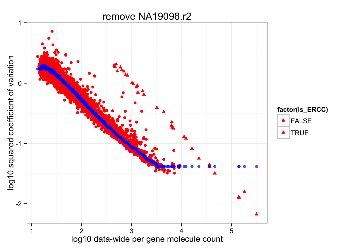
Compute adjusted coefficient of variation.
# adjusted coefficient of variation on log10 scale
log10cv2_adj <-
  lapply(1:length(molecules_cv_batch), function(per_batch) {
    foo <- log10(molecules_cv_batch[[per_batch]]$cv^2) - roll_medians
    return(foo)
})
df_plot$log10cv2_adj <- do.call(c, log10cv2_adj)
df_plot$is_ERCC <- ( 1:dim(df_plot)[1] %in% grep("ERCC", rownames(df_plot)) )
Adjusted squared coefficient of variation versus log10 mean count (CPM corrected).
ggplot( df_plot, aes(x = log10(mean), y = log10cv2_adj) ) +
  geom_point( aes(col = as.factor(batch), shape = factor(is_ERCC)), cex = .9 ) +
  facet_wrap( ~ batch) +
labs(x = "log10(Mean CPM)", y = "log10(Adjusted Squared coefficient of variation") 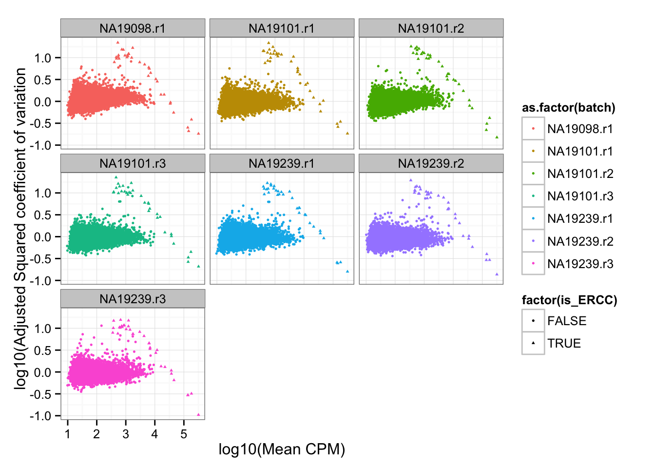
Remove NA19098.r2 + ERCC genes
Remove ERCC genes.
molecules_cv_batch_ENSG <- lapply(1:length(molecules_cv_batch), function(per_batch) {
  obj <- molecules_cv_batch[[per_batch]]
  is_ENSG <- grep("ENSG", rownames(obj))
  obj[is_ENSG, ]
})
Normalize coefficient of variation
Merge summary data.frames.
df_ENSG <- do.call(rbind, molecules_cv_batch_ENSG)Compute rolling medians across all samples.
molecules_all_genes_ENSG <- molecules_all_genes[ grep("ENSG", rownames(molecules_all_genes)) , anno_qc$batch != "NA19098.r1"]

# Compute a data-wide coefficient of variation on CPM normalized counts.
data_cv <- apply(2^molecules_all_genes_ENSG, 1, sd)/apply(2^molecules_all_genes_ENSG, 1, mean)

# Order of genes by mean expression levels
order_gene <- order(apply(2^molecules_all_genes_ENSG, 1, mean))

# Rolling medians of log10 squared CV by mean expression levels
roll_medians <- rollapply(log10(data_cv^2)[order_gene], width = 50, by = 25,
                         FUN = median, fill = list("extend", "extend", "NA") )
ii_na <- which( is.na(roll_medians) )
roll_medians[ii_na] <- median( log10(data_cv^2)[order_gene][ii_na] )

names(roll_medians) <- rownames(molecules_all_genes_ENSG)[order_gene]

# re-order rolling medians
reorder_gene <- match(rownames(molecules_all_genes_ENSG), names(roll_medians) )
head(reorder_gene)
[1] 378 3749 4652 6257 3529 2111roll_medians <- roll_medians[ reorder_gene ]
stopifnot( all.equal(names(roll_medians), rownames(molecules_all_genes_ENSG) ) )Sanity check for the computation of rolling median.
ERCC genes are the outliers in their data-wide average of coefficients of variations. After removing these, the data-wide coefficients of variation look more resonable distributed.
ggplot(data.frame(cv2 = log10(data_cv^2),
                  roll_medians = roll_medians,
                  mean = log10(apply(2^molecules_all_genes_ENSG, 1, mean) ),
                  is_ERCC = (1:length(data_cv) %in% grep("ERCC", names(data_cv)) )  ) ) +
  geom_point( aes(x = mean, y = cv2, shape = factor(is_ERCC) ), col = "red" ) +
  geom_point(aes(x = mean, y = roll_medians), col = "blue", alpha = .7) +
  labs(x = "log10 data-wide per gene molecule count",
       y = "log10 squared coefficient of variation") +
  ggtitle( "remove NA19098.r2, only ENSG")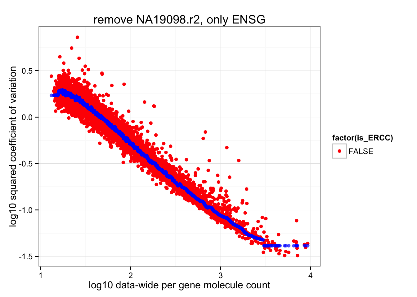
Compute adjusted coefficient of variation.
# adjusted coefficient of variation on log10 scale
log10cv2_adj <-
  lapply(1:length(molecules_cv_batch_ENSG), function(per_batch) {
    foo <- log10(molecules_cv_batch_ENSG[[per_batch]]$cv^2) - roll_medians
    return(foo)
})
df_ENSG$log10cv2_adj <- do.call(c, log10cv2_adj)
df_ENSG$is_ERCC <- ( 1:dim(df_ENSG)[1] %in% grep("ERCC", rownames(df_ENSG)) )
Adjusted squared coefficient of variation versus log10 mean count (CPM corrected).
ggplot( df_ENSG, aes(x = log10(mean), y = log10cv2_adj) ) +
  geom_point( aes(col = as.factor(batch), shape = factor(is_ERCC)), cex = .9 ) +
  facet_wrap( ~ batch) +
labs(x = "log10(Mean CPM)", y = "log10(Adjusted Squared coefficient of variation") 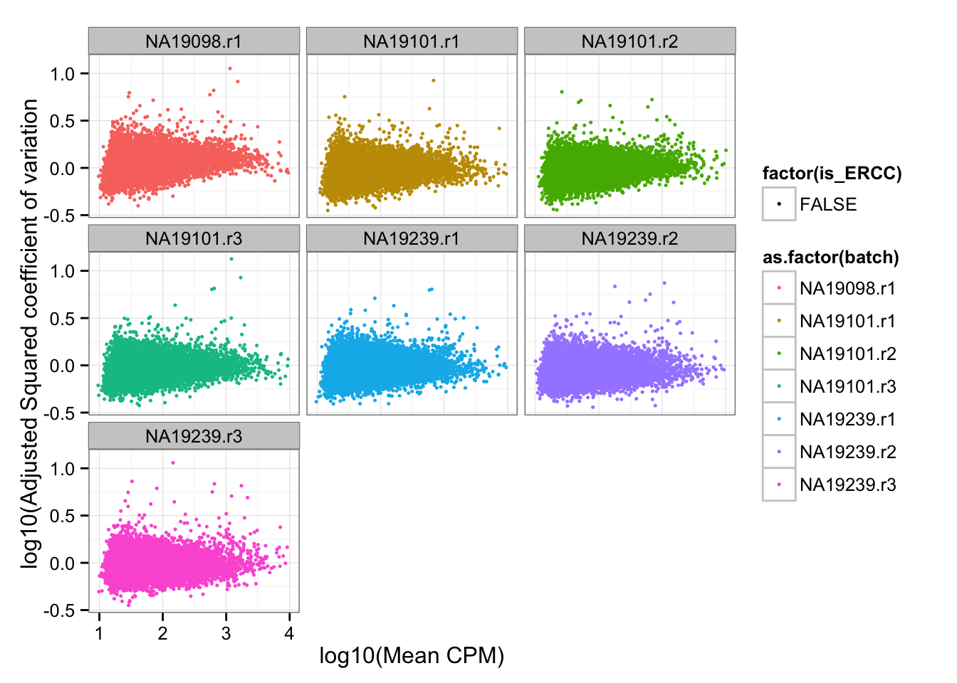
Session information
sessionInfo()R version 3.2.1 (2015-06-18)
Platform: x86_64-apple-darwin13.4.0 (64-bit)
Running under: OS X 10.10.5 (Yosemite)
locale:
[1] en_US.UTF-8/en_US.UTF-8/en_US.UTF-8/C/en_US.UTF-8/en_US.UTF-8
attached base packages:
[1] grid stats graphics grDevices utils datasets methods
[8] base
other attached packages:
[1] zoo_1.7-12 ggplot2_1.0.1 edgeR_3.10.5 limma_3.24.15
[5] dplyr_0.4.3 data.table_1.9.6 knitr_1.11
loaded via a namespace (and not attached):
[1] Rcpp_0.12.2 magrittr_1.5 MASS_7.3-45 munsell_0.4.2
[5] lattice_0.20-33 colorspace_1.2-6 R6_2.1.1 stringr_1.0.0
[9] plyr_1.8.3 tools_3.2.1 parallel_3.2.1 gtable_0.1.2
[13] DBI_0.3.1 htmltools_0.2.6 yaml_2.1.13 assertthat_0.1
[17] digest_0.6.8 reshape2_1.4.1 formatR_1.2.1 evaluate_0.8
[21] rmarkdown_0.8.1 labeling_0.3 stringi_1.0-1 scales_0.3.0
[25] chron_2.3-47 proto_0.3-10