Using ngsplot to calculate coverage over ERCC genes
2015-03-15
Last updated: 2016-03-15
Code version: 1db9308a307e8e4185c5d233188ba21e5996e560
Here I use ngsplot to calculate coverage.
Conclusions:
- The coverage across the ERCC genes is uniform with a 3’ increase
- Though minimal, there is unexpected coverage in the antisense direction
- The majority of the signal is coming from the highest expressed genes
- When split by length, the shortest and longest genes contribute most to the coverage signal
Since the ERCC are quite short, I use a fragment length of 50. The endogenous analysis used a fragment length of 100.
library("tidyr")
library("ggplot2")
library("cowplot")
theme_set(theme_bw(base_size = 12))
theme_update(panel.grid.minor.x = element_blank(),
             panel.grid.minor.y = element_blank(),
             panel.grid.major.x = element_blank(),
             panel.grid.major.y = element_blank())
Functions
The following function aggregate results from the various ngsplot runs.
import_ngsplot <- function(results, id = 1:length(results)) {
  # Imports and combines results from multiple ngsplot analyses
  #
  # results - name of ngsplot results (specified with -O flag)
  # id - description of analysis
  library("tidyr")
  stopifnot(length(results) > 0, length(results) == length(id))
  avgprof_list <- list()
  sem_list <- list()
  for (i in seq_along(results)) {
    zipfile <- paste0(results[i], ".zip")
    extract_zip(zipfile)
    # Import mean coverage
    avgprof_list[[i]] <- import_data(path = results[i], datatype = "avgprof",
                                     id = id[i])
    # Import standard error of mean coverage
    sem_list[[i]] <- import_data(path = results[i], datatype = "sem",
                                 id = id[i])
  }
  avgprof_df <- do.call(rbind, avgprof_list)
  sem_df <- do.call(rbind, sem_list)
  final <- merge(avgprof_df, sem_df)
  return(final)
}

extract_zip <- function(zipfile) {
  # Unzip the ngsplot results into the same directory
  stopifnot(length(zipfile) == 1, file.exists(zipfile))
  unzip(zipfile, exdir = dirname(zipfile))
  return(invisible())
}

import_data <- function(path, datatype, id) {
  # Import the data from a specific ngsplot file.
  #
  # path - path to the ngsplot results directory
  # datatype - either "avgprof" for the mean coverage or
  #            "sem" for the standard error of the mean coverage
  # id - description of analysis (length == 1)
  stopifnot(datatype == "avgprof" | datatype == "sem",
            length(id) == 1)
  fname <- paste0(path, "/", datatype, ".txt")
  df <- read.delim(fname)
  df$position <- paste0("p", 1:nrow(df))
  df$id <- id
  df_long <- gather_(df, key_col = "metainfo", value = datatype)
  df_long$metainfo <- as.character(df_long$metainfo)
  df_long$position <- sub("^p", "", df_long$position)
  df_long$position <- as.numeric(df_long$position)
  return(df_long)
}
Coverage
First I observe the coverage for all filtered ERCC genes.
Unzip and import the raw coverage data.
cov <- import_ngsplot(results = c("../data/ngsplot-molecules-ercc-both",
                                  "../data/ngsplot-molecules-ercc-same",
                                  "../data/ngsplot-molecules-ercc-opposite"),
                      id = c("ercc-both",
                             "ercc-same",
                             "ercc-opposite"))
Using position, id as id variables
Using position, id as id variables
Using position, id as id variables
Using position, id as id variables
Using position, id as id variables
Using position, id as id variablescov <- separate(cov, "id", into = c("feature", "strand"), sep = "-")Plotting results.
p <- ggplot(NULL, aes(x = position, y = avgprof, color = metainfo)) +
  geom_line()+
  geom_ribbon(aes(ymin = avgprof - sem, ymax = avgprof + sem,
                  color = NULL, fill = metainfo), alpha = 0.25) +
  geom_vline(x = c(20, 80), color = "grey") +
  scale_x_continuous(breaks = c(0, 20, 40, 60, 80, 100),
                     labels = c(-100, "TSS", "33%", "66%", "TES", 100)) +
  facet_wrap(~strand, ncol = 1, scales = "free_y") +
  theme(legend.position = "none") +
  labs(x = "Position", y = "Mean molecules per million")
plot_ercc <- p %+% cov + labs(title = "ERCC")Plot
Note the smaller y-axis for the opposite strand. While it is very small compared to the sense strand, I highlight it because we expect no reads mapping in the antisense direction.
plot_ercc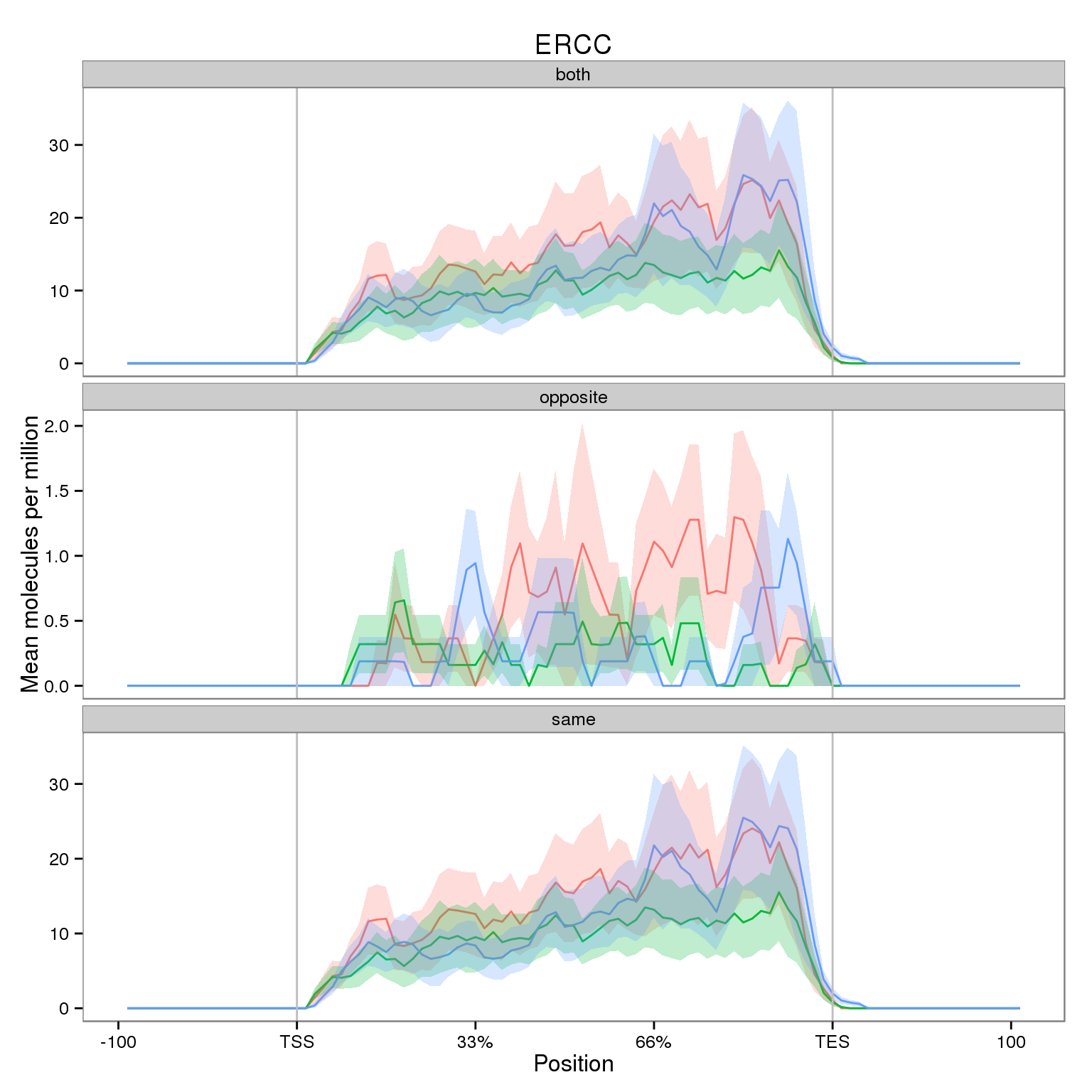
Coverage by expression level
Next I compare the coverage for NA19091 for genes split into expression quartiles.
cov_expr <- import_ngsplot(results = c("../data/ngsplot-ercc-expr-both",
                                       "../data/ngsplot-ercc-expr-same",
                                       "../data/ngsplot-ercc-expr-opposite"),
                           id = c("both", "same", "opposite"))
Using position, id as id variables
Using position, id as id variables
Using position, id as id variables
Using position, id as id variables
Using position, id as id variables
Using position, id as id variablescolnames(cov_expr)[colnames(cov_expr) == "id"] <- "strand"Plot
plot_expr <- plot_ercc %+% cov_expr +
  scale_color_discrete(name = "Expression quartile") +
  scale_fill_discrete(name = "Expression quartile") +
  theme(legend.position = "bottom")
plot_expr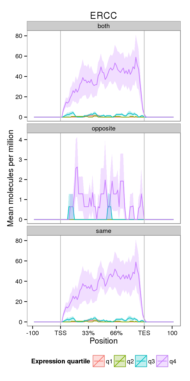
Notice the increased y-axis.
Coverage by gene length
Next I compare the coverage for NA19091 for genes split by gene length.
cov_len <- import_ngsplot(results = c("../data/ngsplot-ercc-len-both",
                                  "../data/ngsplot-ercc-len-same",
                                  "../data/ngsplot-ercc-len-opposite"),
                      id = c("both", "same", "opposite"))
Using position, id as id variables
Using position, id as id variables
Using position, id as id variables
Using position, id as id variables
Using position, id as id variables
Using position, id as id variablescolnames(cov_len)[colnames(cov_len) == "id"] <- "strand"Plot
plot_len <- plot_ercc %+% cov_len +
  scale_color_discrete(name = "Length quartile") +
  scale_fill_discrete(name = "Length quartile") +
  theme(legend.position = "bottom")
plot_len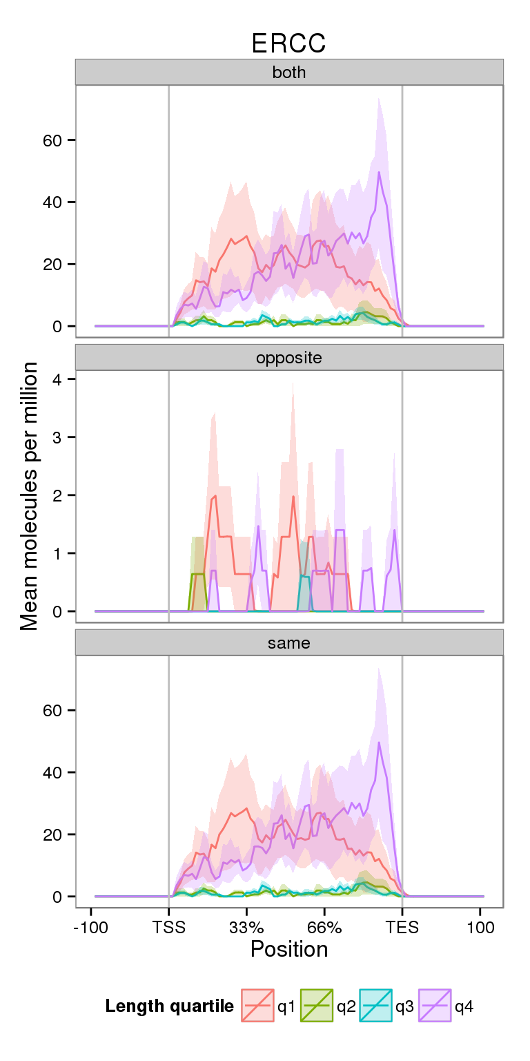
Session information
sessionInfo()R version 3.2.0 (2015-04-16)
Platform: x86_64-unknown-linux-gnu (64-bit)
locale:
[1] LC_CTYPE=en_US.UTF-8 LC_NUMERIC=C
[3] LC_TIME=en_US.UTF-8 LC_COLLATE=en_US.UTF-8
[5] LC_MONETARY=en_US.UTF-8 LC_MESSAGES=en_US.UTF-8
[7] LC_PAPER=en_US.UTF-8 LC_NAME=C
[9] LC_ADDRESS=C LC_TELEPHONE=C
[11] LC_MEASUREMENT=en_US.UTF-8 LC_IDENTIFICATION=C
attached base packages:
[1] stats graphics grDevices utils datasets methods base
other attached packages:
[1] cowplot_0.3.1 ggplot2_1.0.1 tidyr_0.2.0 knitr_1.10.5
[5] rmarkdown_0.6.1
loaded via a namespace (and not attached):
[1] Rcpp_0.12.0 magrittr_1.5 MASS_7.3-40 munsell_0.4.2
[5] colorspace_1.2-6 stringr_1.0.0 httr_0.6.1 plyr_1.8.3
[9] tools_3.2.0 grid_3.2.0 gtable_0.1.2 htmltools_0.2.6
[13] yaml_2.1.13 digest_0.6.8 reshape2_1.4.1 formatR_1.2
[17] bitops_1.0-6 RCurl_1.95-4.6 evaluate_0.7 labeling_0.3
[21] stringi_0.4-1 scales_0.2.4 proto_0.3-10