Identification of noisy genes
Po-Yuan Tung
2015-06-03
Last updated: 2015-06-29
Code version: e927fac891c5ab5af9b62b9eecc0232855931c96
Input
library("dplyr")
library("ggplot2")
theme_set(theme_bw(base_size = 16))
library("edgeR")
Summary counts from featureCounts. Created with gather-summary-counts.py.
summary_counts <- read.table("../data/summary-counts.txt", header = TRUE,
                             stringsAsFactors = FALSE)
summary_per_sample <- summary_counts %>%
  filter(sickle == "quality-trimmed") %>%
  select(-sickle) %>%
  arrange(individual, batch, well, rmdup) %>%
  as.data.frame
Input annotation.
anno <- read.table("../data/annotation.txt", header = TRUE,
                   stringsAsFactors = FALSE)
head(anno)
individual batch well sample_id
1 19098 1 A01 NA19098.1.A01
2 19098 1 A02 NA19098.1.A02
3 19098 1 A03 NA19098.1.A03
4 19098 1 A04 NA19098.1.A04
5 19098 1 A05 NA19098.1.A05
6 19098 1 A06 NA19098.1.A06Input read counts.
reads <- read.table("../data/reads.txt", header = TRUE,
                    stringsAsFactors = FALSE)
Input molecule counts.
molecules <- read.table("../data/molecules.txt", header = TRUE,
                    stringsAsFactors = FALSE)
Input single cell observational quality control data.
qc <- read.table("../data/qc-ipsc.txt", header = TRUE,
                 stringsAsFactors = FALSE)
head(qc)
individual batch well cell_number concentration tra1.60
1 19098 1 A01 1 1.734785 1
2 19098 1 A02 1 1.723038 1
3 19098 1 A03 1 1.512786 1
4 19098 1 A04 1 1.347492 1
5 19098 1 A05 1 2.313047 1
6 19098 1 A06 1 2.056803 1Input list of single cells to keep based on qc.
goodcell <- read.table("../data/quality-single-cells.txt", header = TRUE,
                 stringsAsFactors = FALSE)
head(goodcell)
NA19098.1.A01
1 NA19098.1.A02
2 NA19098.1.A05
3 NA19098.1.A06
4 NA19098.1.A07
5 NA19098.1.A08
6 NA19098.1.A10Remove bad quality cells
Remove cells with total reads < 2 millons
#reads per sample
summary_per_sample_reads <- summary_per_sample %>% filter(rmdup == "reads")

#create unmapped ratios
summary_per_sample_reads$unmapped.ratios <- summary_per_sample_reads[,9]/apply(summary_per_sample_reads[,5:13],1,sum)

#create total mapped reads
summary_per_sample_reads$total.mapped <- apply(summary_per_sample_reads[,5:8],1,sum)

#creat ERCC ratios
summary_per_sample_reads$ERCC.ratios <- apply(reads[grep("ERCC", rownames(reads)), ],2,sum)/apply(summary_per_sample_reads[,5:8],1,sum)

#remove bulk keep single cell
summary_per_sample_reads_single <- summary_per_sample_reads[summary_per_sample_reads$well!="bulk",]

#add cell number per well by merging qc file
summary_per_sample_reads_single_qc <- merge(summary_per_sample_reads_single,qc,by=c("individual","batch","well"))

#qc filter
summary_per_sample_reads_single_qc$qc_filter <- summary_per_sample_reads_single_qc$cell_number == 1 & summary_per_sample_reads_single_qc$total.mapped > 2 * 10^6

sum(summary_per_sample_reads_single_qc$qc_filter)
[1] 632ggplot(summary_per_sample_reads_single_qc, aes(x = total.mapped , y = unmapped.ratios, col = qc_filter)) + geom_text(aes(label = cell_number))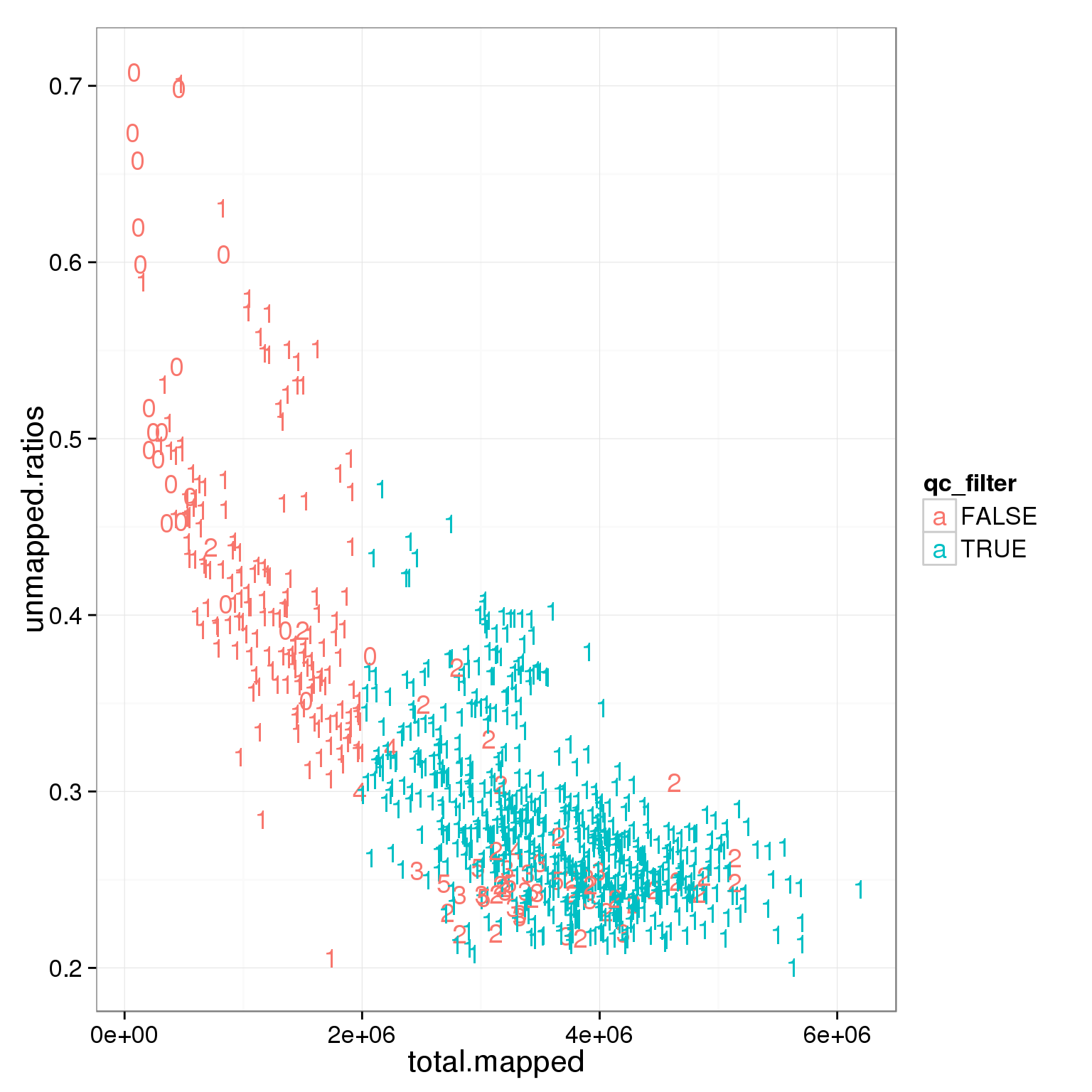
ggplot(summary_per_sample_reads_single_qc, aes(x = total.mapped , y = ERCC.ratios, col = qc_filter)) + geom_text(aes(label = cell_number))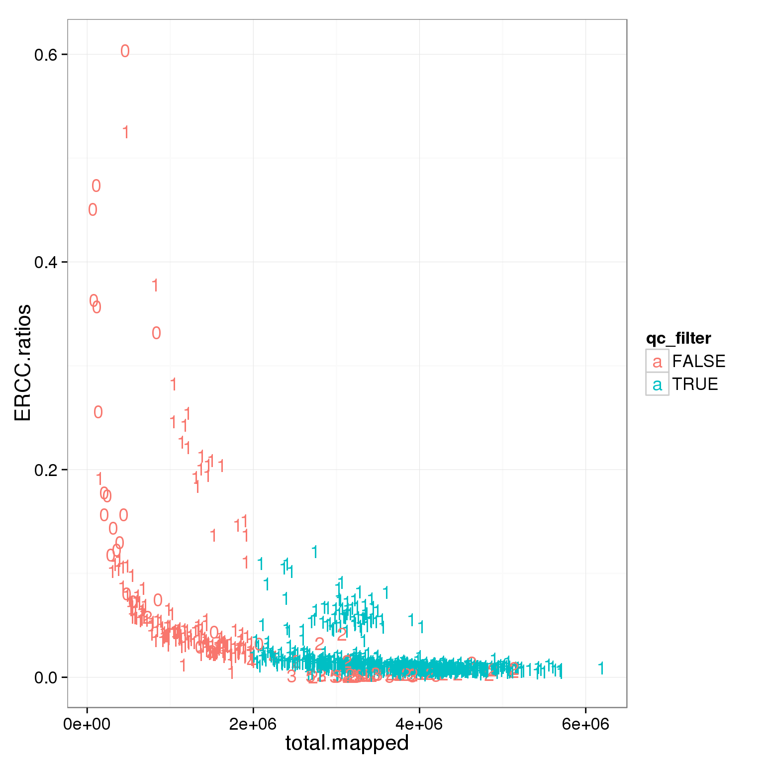
Total molecule number of ERCC
# molecules per sample
summary_per_sample_molecules <- summary_per_sample %>% filter(rmdup == "molecules")

# total ERCC molecule
summary_per_sample_molecules$total.ERCC.mol <- apply(molecules[grep("ERCC", rownames(reads)), ],2,sum)

# ERCC molecule ratio
summary_per_sample_molecules$ERCC.ratio.mol <- summary_per_sample_molecules$total.ERCC.mol/summary_per_sample_molecules$Assigned

# remove bulk keep single cell
summary_per_sample_molecules_single <- summary_per_sample_molecules[summary_per_sample_molecules$well!="bulk",]

plot(summary_per_sample_molecules_single$total.ERCC.mol)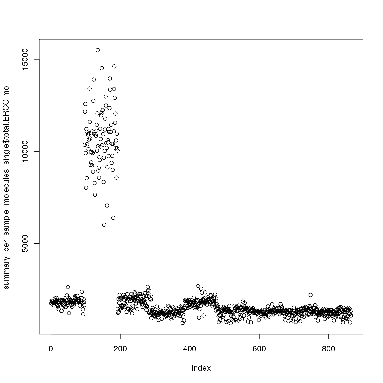
# adjust total ERCC molecules of 19098 batch2
summary_per_sample_molecules_single$index_19098_2 <- (summary_per_sample_molecules_single$individual == "19098" & summary_per_sample_molecules_single$batch == "2")

# calculating the ratio of 19098 batch 2 to the rest
adjusted_ratio.mol <- mean(summary_per_sample_molecules_single$total.ERCC.mol[summary_per_sample_molecules_single$index_19098_2])/mean(summary_per_sample_molecules_single$total.ERCC[!summary_per_sample_molecules_single$index_19098_2])

adjusted_ratio.mol
[1] 7.287311# adjusted total ERCC reads
summary_per_sample_molecules_single$adj.total.ERCC.mol <- summary_per_sample_molecules_single$total.ERCC.mol
summary_per_sample_molecules_single$adj.total.ERCC.mol[summary_per_sample_molecules_single$index_19098_2] <- summary_per_sample_molecules_single$adj.total.ERCC.mol[summary_per_sample_molecules_single$index_19098_2]/adjusted_ratio.mol
# adjusted ERCC ratios
summary_per_sample_molecules_single$adj.ERCC.ratios.mol <-
summary_per_sample_molecules_single$adj.total.ERCC.mol/summary_per_sample_molecules_single$Assigned
# add qc filter and cell number
summary_per_sample_molecules_single$qc_filter <- summary_per_sample_reads_single_qc$qc_filter
summary_per_sample_molecules_single$cell_number <- summary_per_sample_reads_single_qc$cell_number
ggplot(summary_per_sample_molecules_single, aes(x = Assigned, y = ERCC.ratio.mol, col = qc_filter)) + geom_text(aes(label = cell_number)) + facet_grid(individual ~ batch) + theme(axis.text.x = element_text(angle = 90, hjust = 0.9, vjust = 0.5))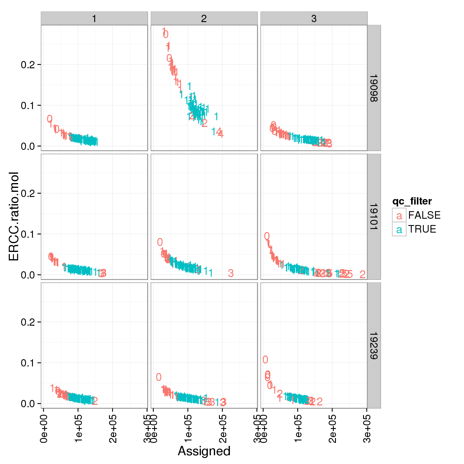
ggplot(summary_per_sample_molecules_single, aes(x = Assigned, y = adj.ERCC.ratios.mol, col = qc_filter)) + geom_text(aes(label = cell_number)) + facet_grid(individual ~ batch) + theme(axis.text.x = element_text(angle = 90, hjust = 0.9, vjust = 0.5))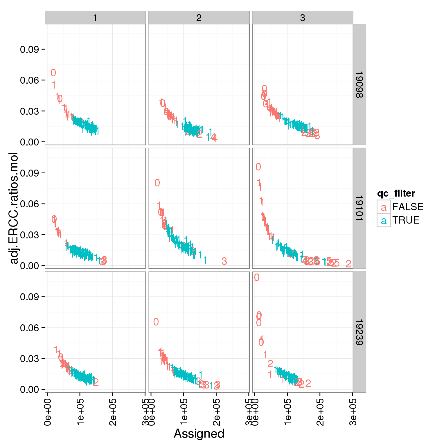
CV and mean
Looking at molecule
# remove molecules that are larger than 1024
rownames(molecules)[rowMeans(molecules) > 1024]
[1] "ENSG00000198712" "ENSG00000198938"molecules.new <- molecules [rowMeans(molecules) < 1024,]
dim(molecules)[1] 20419 873dim(molecules.new)[1] 20417 873# remove bulk
molecules_single <- molecules %>% select(-contains("bulk"))
# remove 1024 and greater
molecules_single <- molecules_single[apply(molecules_single,1,max) < 1024,]
# apply qc_filter
molecules_single_qc <- molecules_single[,summary_per_sample_reads_single_qc$qc_filter]
dim(molecules_single_qc)[1] 20396 632sample_name <- names(molecules_single_qc)
### create a function to compute the cv and mean of molecules
### input data is molecules_single_qc
### two parameters
### 1. filter: sellect for specifc individaul or batch
### 2. adj.19098.batch: flag to control if we want to adj the 19098 batch2 molecules numberes. default to not adj, meaning using the raw numbers
prep_molecules.cv.mean <- function(filter,adj.19098.batch2=0){
### generate the data of interest
data.in <- molecules_single_qc[,grepl(filter,sample_name)]
if(adj.19098.batch2 == 1){
#### find out which columns belong 19098 batch2
target.column <- sample_name[grep("19098.2",sample_name)]
#### find out ERCC rows
g <- rownames(data.in)
target.row <- g[grep("ERCC",g)]
#### replace the molecules numbers via dividing by adjusted_ratio.mol
data.in[target.row,target.column] <- (data.in[target.row,target.column])/adjusted_ratio.mol
}
if(adj.19098.batch2 == 2){
#### find out which columns belong 19098 batch2
#### remove 19098.2
data.in<- data.in[,!grepl("19098.2",sample_name)]
#### also need to take care of summary_per_sample_reads_single_qc
summary_per_sample_reads_single_qc <- summary_per_sample_reads_single_qc[!((summary_per_sample_reads_single_qc$individual==19098)&(summary_per_sample_reads_single_qc$batch==2)),]
}
if(adj.19098.batch2 == 3){
#### find out which columns belong 19098 batch2
target.column <- sample_name[grep("19098.2",sample_name)]
#### find out ERCC rows
g <- rownames(data.in)
target.row <- g[grep("ERCC",g)]
#### replace the molecules numbers with NA
data.in[target.row,target.column] <- NA
}
#correct for collision probability
molecules.crt <- -1024*log(1-data.in/1024)
# create a new dataset
molecules_single_qc_w_mean_cv <- molecules.crt
# add mean
molecules_single_qc_w_mean_cv$mean <- apply(molecules.crt, 1, function(x) mean(x,na.rm=TRUE) )
# add CV
molecules_single_qc_w_mean_cv$CV <- apply(molecules.crt, 1, function(x) sd(x,na.rm=TRUE) )/ apply(molecules.crt, 1, function(x) mean(x,na.rm=TRUE))
# add variance
molecules_single_qc_w_mean_cv$var <- apply(molecules.crt, 1, function(x) var(x,na.rm=TRUE) )
# remove non-expressed
molecules_single_qc_expressed <- molecules_single_qc_w_mean_cv[molecules_single_qc_w_mean_cv$mean >0,]
dim(molecules_single_qc_expressed)
# create a flag to ERCC
molecules_single_qc_expressed$ERCC <- grepl("ERCC",rownames(molecules_single_qc_expressed))
# add gene_name
molecules_single_qc_expressed$gene_name <- rownames(molecules_single_qc_expressed)
return(molecules_single_qc_expressed)
### end of prep.molecules.cv.mean function
}
molecules_single_qc_expressed <- prep_molecules.cv.mean(filter="19",adj.19098.batch2=0)
molecules_single_qc_expressed_adj <- prep_molecules.cv.mean(filter="19",adj.19098.batch2=1)
molecules_single_qc_expressed_rm <- prep_molecules.cv.mean(filter="19",adj.19098.batch2=2)
molecules_single_qc_expressed_rm_ERCC <- prep_molecules.cv.mean(filter="19",adj.19098.batch2=3)
# plot with color-blind-friendly palettes
cbPalette <- c("#999999", "#0000FF", "#56B4E9", "#009E73", "#F0E442", "#0072B2", "#D55E00", "#CC79A7")
ggplot(molecules_single_qc_expressed, aes(x = mean, y = CV, col = ERCC)) + geom_point(size = 2, alpha = 0.5) + scale_x_log10() + scale_colour_manual(values=cbPalette)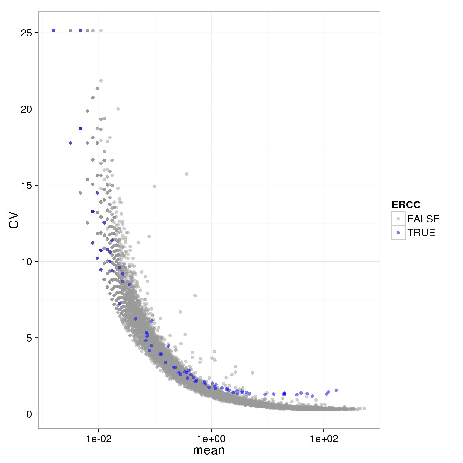
ggplot(molecules_single_qc_expressed_rm_ERCC, aes(x = mean, y = CV, col = ERCC)) + geom_point(size = 2, alpha = 0.5) + scale_x_log10() + scale_colour_manual(values=cbPalette)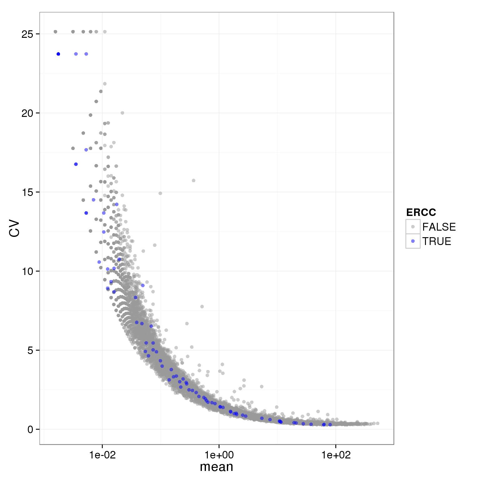
### create molecule data by each individaul using the molecules_single_qc_expressed_rm_ERCC
## 19098
individual_19098_mean_CV <- prep_molecules.cv.mean(filter="19098",adj.19098.batch2 = 0)

ggplot(individual_19098_mean_CV, aes(x = mean, y = CV, col = ERCC))  + geom_point(size = 2, alpha = 0.5) + scale_x_log10() + scale_colour_manual(values=cbPalette)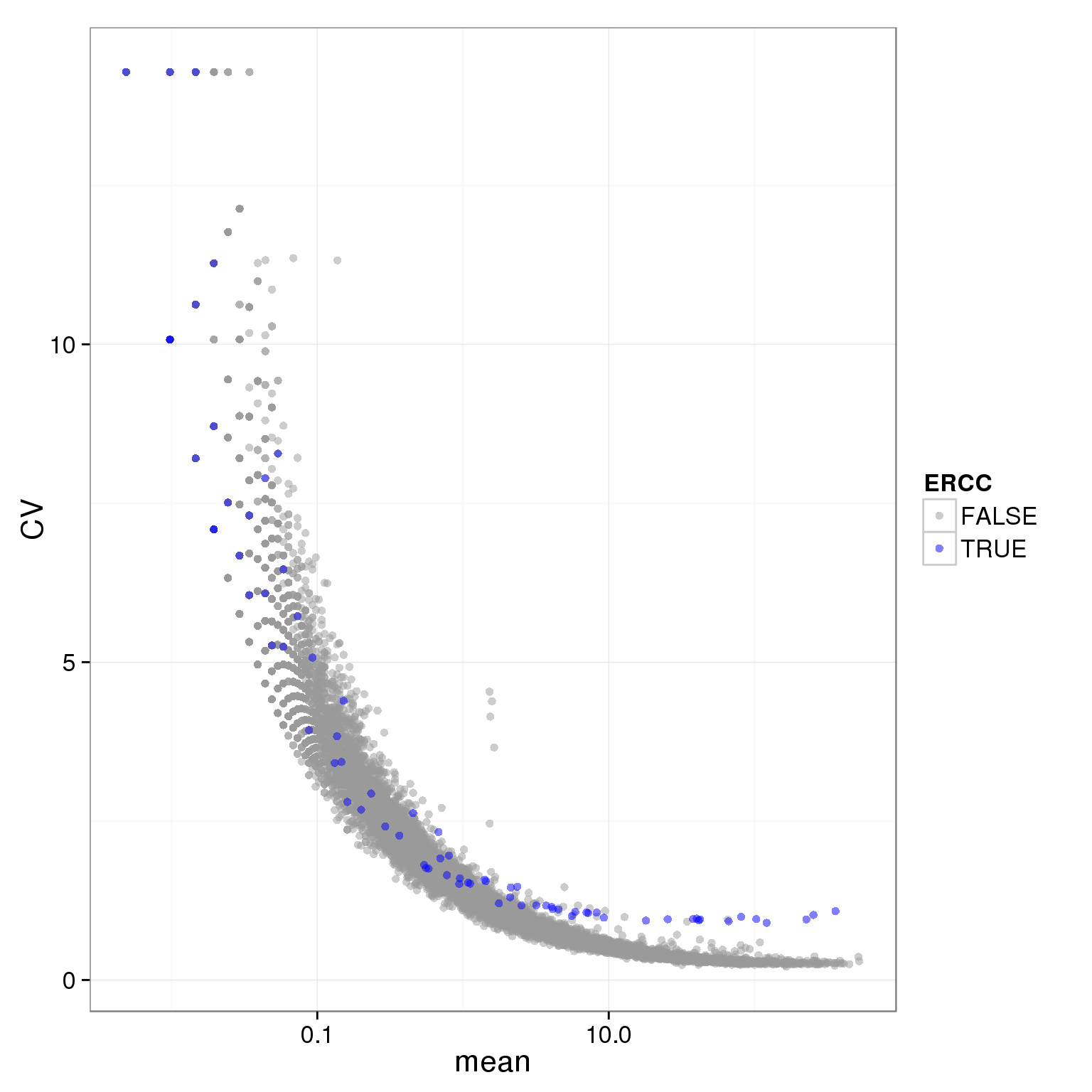
## 19101
individual_19101_mean_CV <- prep_molecules.cv.mean(filter="19101",adj.19098.batch2 = 0)

ggplot(individual_19101_mean_CV, aes(x = mean, y = CV, col = ERCC))  + geom_point(size = 2, alpha = 0.5) + scale_x_log10() + scale_colour_manual(values=cbPalette)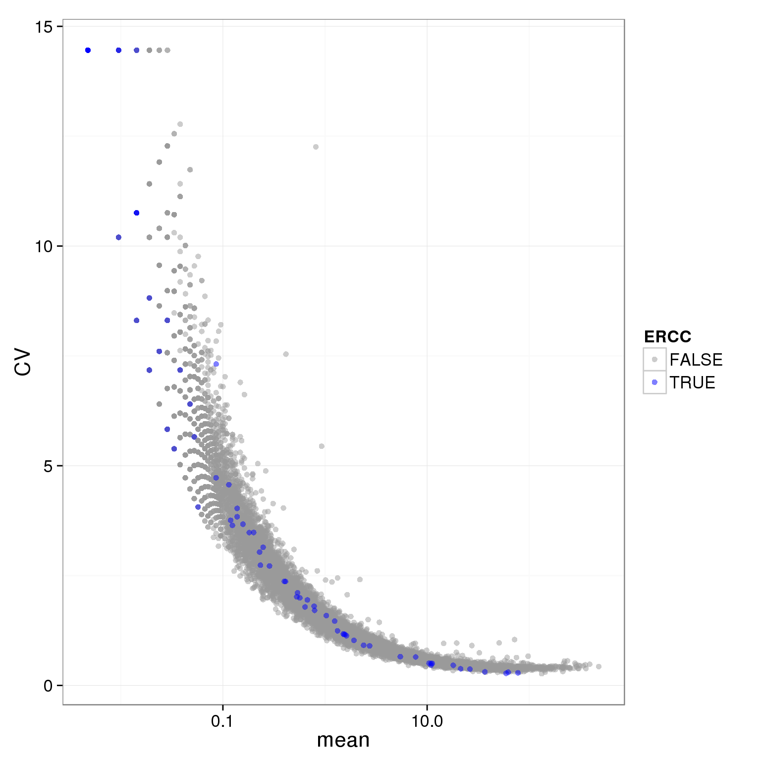
## 19239
individual_19239_mean_CV <- prep_molecules.cv.mean(filter="19239",adj.19098.batch2 = 0)

ggplot(individual_19239_mean_CV, aes(x = mean, y = CV, col = ERCC))  + geom_point(size = 2, alpha = 0.5) + scale_x_log10() + scale_colour_manual(values=cbPalette)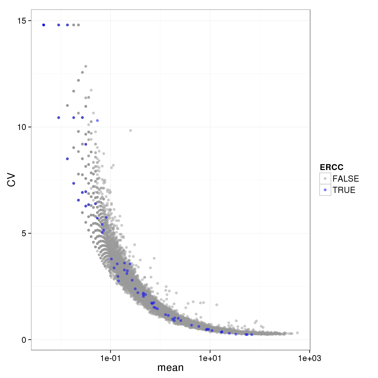
Looking at reads
# remove bulk
reads_single <- reads %>% select(-contains("bulk"))

# apply qc_filter
reads_single_qc <- reads_single[,summary_per_sample_reads_single_qc$qc_filter]
dim(reads_single_qc)
[1] 20419 632sum(summary_per_sample_reads_single_qc$qc_filter)[1] 632# normalization
reads_single_qc_cpm <- cpm(reads_single_qc)
# create a new dataset
reads_single_qc_w_mean_cv <- data.frame(reads_single_qc_cpm)
sum(reads_single_qc_cpm!=reads_single_qc_w_mean_cv)[1] 0# add mean
reads_single_qc_w_mean_cv$mean <- apply(reads_single_qc_cpm, 1, mean)
# add CV
reads_single_qc_w_mean_cv$CV <- apply(reads_single_qc_cpm, 1, sd)/ apply(reads_single_qc_cpm, 1, mean)
# remove non-expressed
reads_single_qc_expressed <- reads_single_qc_w_mean_cv[reads_single_qc_w_mean_cv$mean >0,]
dim(reads_single_qc_expressed)[1] 17609 634# sellect ERCC
reads_single_qc_expressed$ERCC <- grepl("ERCC",rownames(reads_single_qc_expressed))
# plot with color-blind-friendly palettes
cbPalette <- c("#999999", "#0000FF", "#56B4E9", "#009E73", "#F0E442", "#0072B2", "#D55E00", "#CC79A7")
ggplot(reads_single_qc_expressed, aes(x = mean, y = CV, col = ERCC)) + geom_point(size = 2, alpha = 0.5) + scale_x_log10() + scale_colour_manual(values=cbPalette)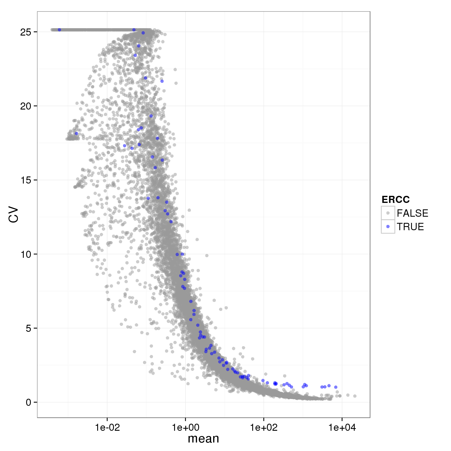
Poisson sucks!
### this function will plot the mean vs cv based on the ERCC molecules counts
### only need to specify the input dataset
### the inpute dataset needs to have mean, cv and ERCC flag
### make minipar global
plot.cv.and.mean <- function(data.in){
    # model based on ERCC only
    # need to have a ERCC flag on the data.in
    molecules_single_qc_expressed_ERCC <- data.in[data.in$ERCC,]

    # defnine poisson function on a log x scale
    poisson.c <- function (x) {
        (10^x)^(0.5)/(10^x)
    }

    # compute the lossy factor based on ERCC
    ####   use LS: first define the function of f, then find the minimum
    ####   dont use the points from ERCC.mol.mean < 0.1 to fit.

    ERCC.mol.mean <- molecules_single_qc_expressed_ERCC$mean
    ERCC.mol.CV   <- molecules_single_qc_expressed_ERCC$CV

    # compute the sum of square errors
    target.fun <- function(f){
        sum((ERCC.mol.CV[ERCC.mol.mean>0.1]- sqrt(1/(f*ERCC.mol.mean[ERCC.mol.mean>0.1])))^2)
    }
    # find out the minimum
    ans <- nlminb(0.05,target.fun,lower=0.0000001,upper=1)
    minipar <- ans$par
    # use the minimum to create the lossy poisson
    lossy.posson <- function (x) {
        1/sqrt((10^x)*minipar)
    }

    # 4 s.d.
    four.sd <- function (x) {
        4*(10^x)^(0.5)/(10^x)
    }

    # 3.7 sd + 0.3
    three.sd <- function (x) {
        3.7*(10^x)^(0.5)/(10^(x))+0.3
    }

    ggplot(data.in, aes(x = mean, y = CV, col = ERCC))  + geom_point(size = 2, alpha = 0.5) +  stat_function(fun= poisson.c, col= "#CC79A7") + stat_function(fun= four.sd, col= "#F0E442") + stat_function(fun= lossy.posson, col= "#56B4E9") + scale_x_log10() + ylim(0, max(data.in$CV)*1.1) + scale_colour_manual(values=cbPalette) + xlab("Average number of molecules") + ylab ("coefficient of variation (CV)")

}
plot.cv.and.mean(data.in=molecules_single_qc_expressed)
Warning in loop_apply(n, do.ply): Removed 21 rows containing missing values
(geom_path).Warning in loop_apply(n, do.ply): Removed 7 rows containing missing values
(geom_path).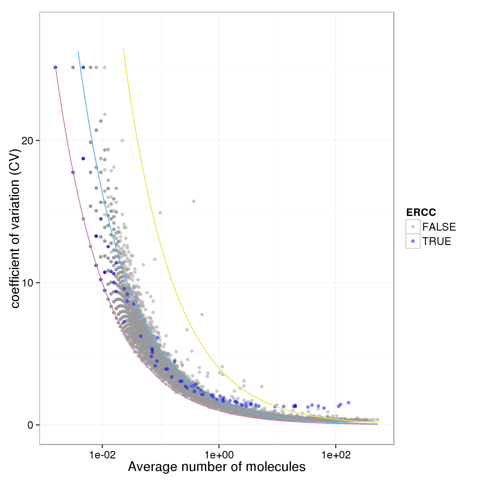
plot.cv.and.mean(data.in=molecules_single_qc_expressed_adj)Warning in loop_apply(n, do.ply): Removed 6 rows containing missing values
(geom_path).Warning in loop_apply(n, do.ply): Removed 26 rows containing missing values
(geom_path).Warning in loop_apply(n, do.ply): Removed 10 rows containing missing values
(geom_path).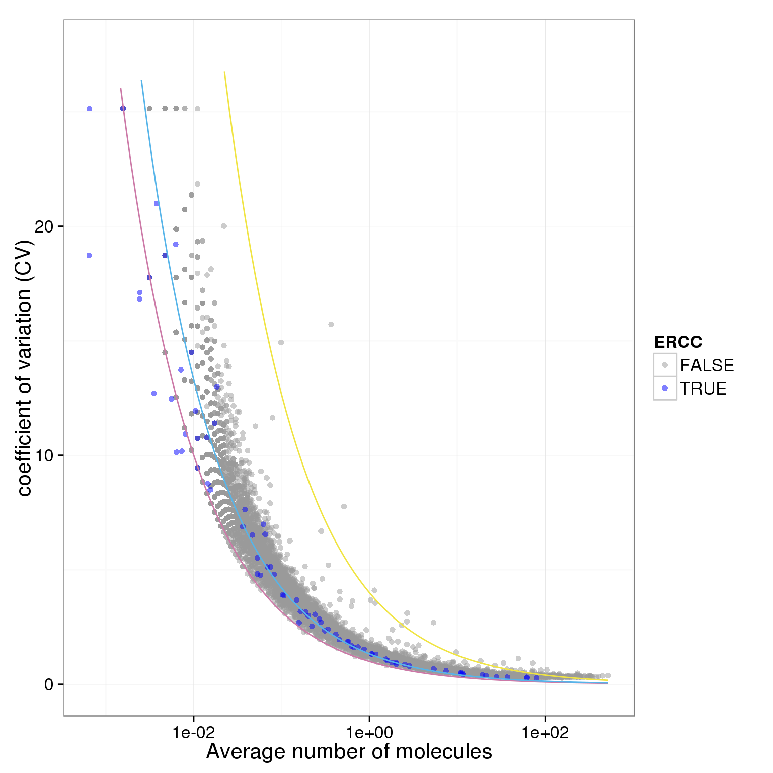
plot.cv.and.mean(data.in=molecules_single_qc_expressed_rm)Warning in loop_apply(n, do.ply): Removed 21 rows containing missing values
(geom_path).Warning in loop_apply(n, do.ply): Removed 4 rows containing missing values
(geom_path).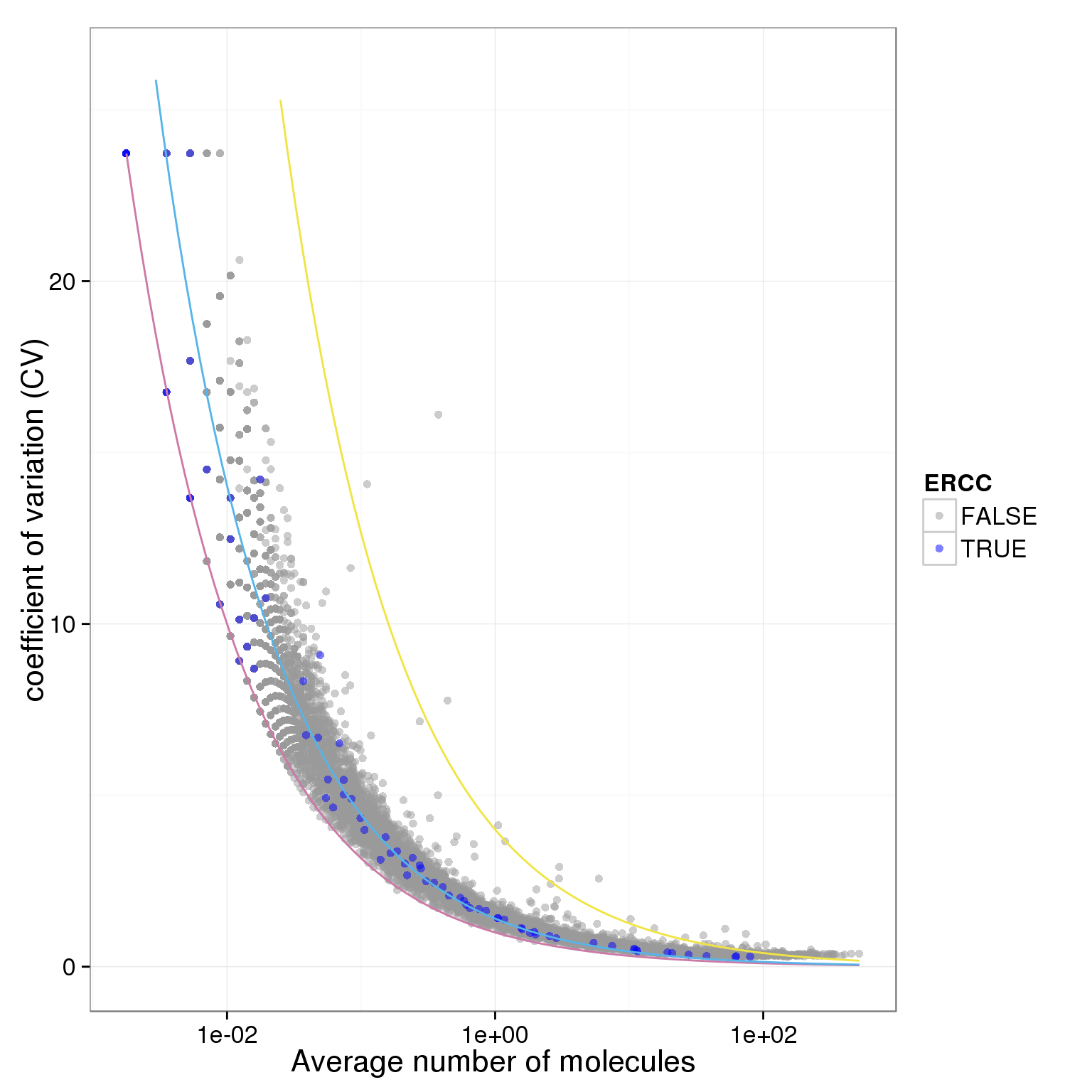
plot.cv.and.mean(data.in=molecules_single_qc_expressed_rm_ERCC)Warning in loop_apply(n, do.ply): Removed 21 rows containing missing values
(geom_path).Warning in loop_apply(n, do.ply): Removed 4 rows containing missing values
(geom_path).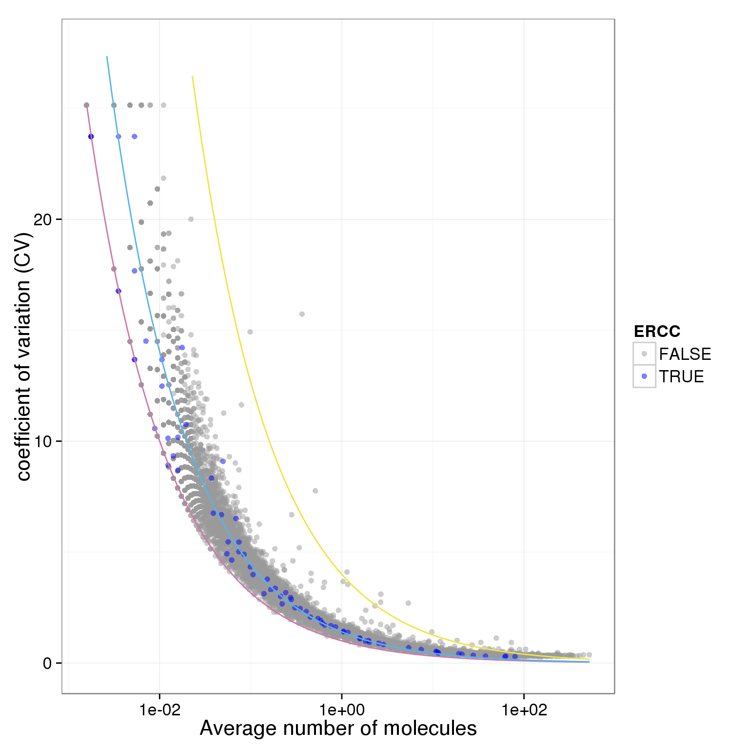
plot.cv.and.mean(data.in=individual_19098_mean_CV)Warning in loop_apply(n, do.ply): Removed 23 rows containing missing values
(geom_path).Warning in loop_apply(n, do.ply): Removed 6 rows containing missing values
(geom_path).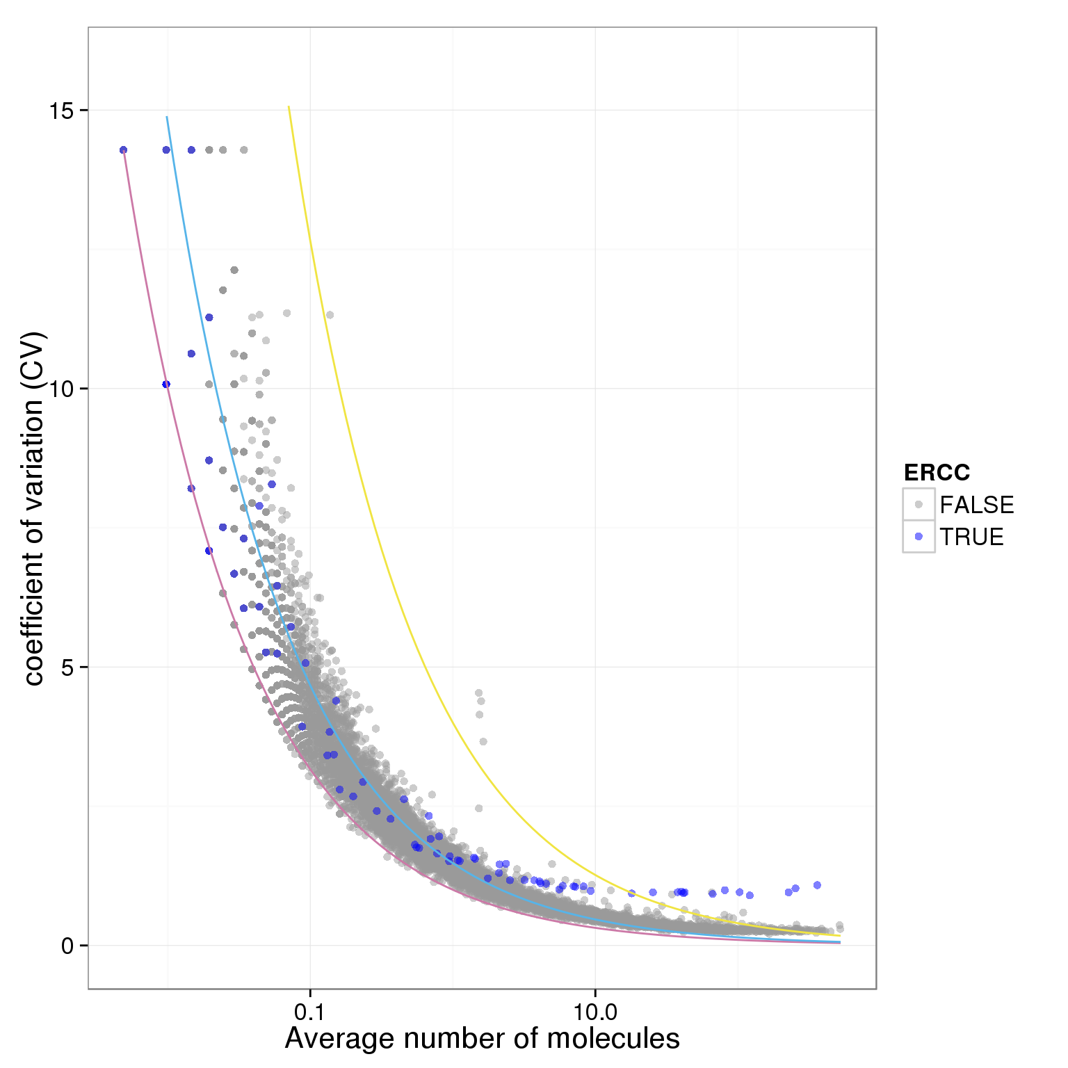
plot.cv.and.mean(data.in=individual_19101_mean_CV)Warning in loop_apply(n, do.ply): Removed 23 rows containing missing values
(geom_path).Warning in loop_apply(n, do.ply): Removed 5 rows containing missing values
(geom_path).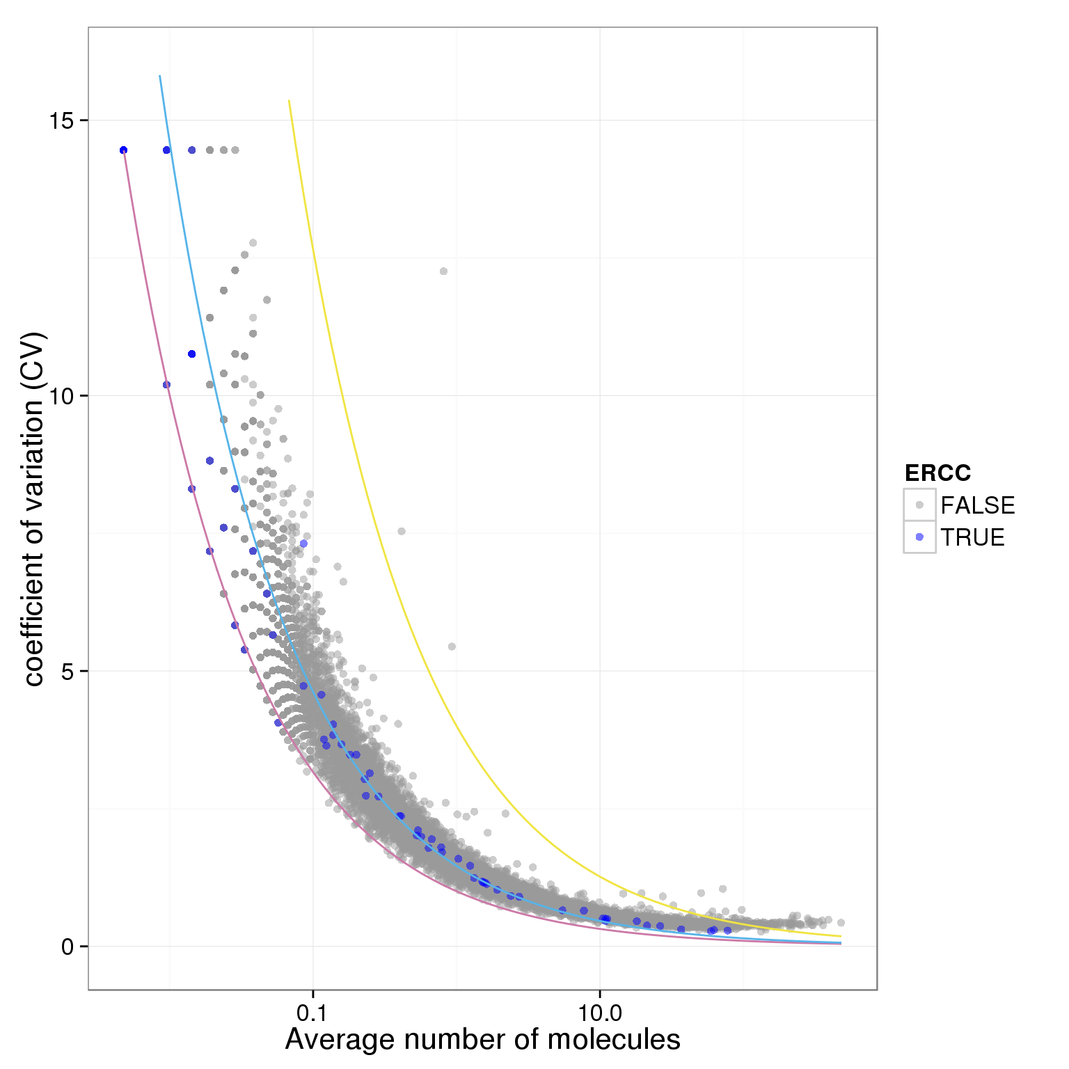
plot.cv.and.mean(data.in=individual_19239_mean_CV)Warning in loop_apply(n, do.ply): Removed 22 rows containing missing values
(geom_path).Warning in loop_apply(n, do.ply): Removed 4 rows containing missing values
(geom_path).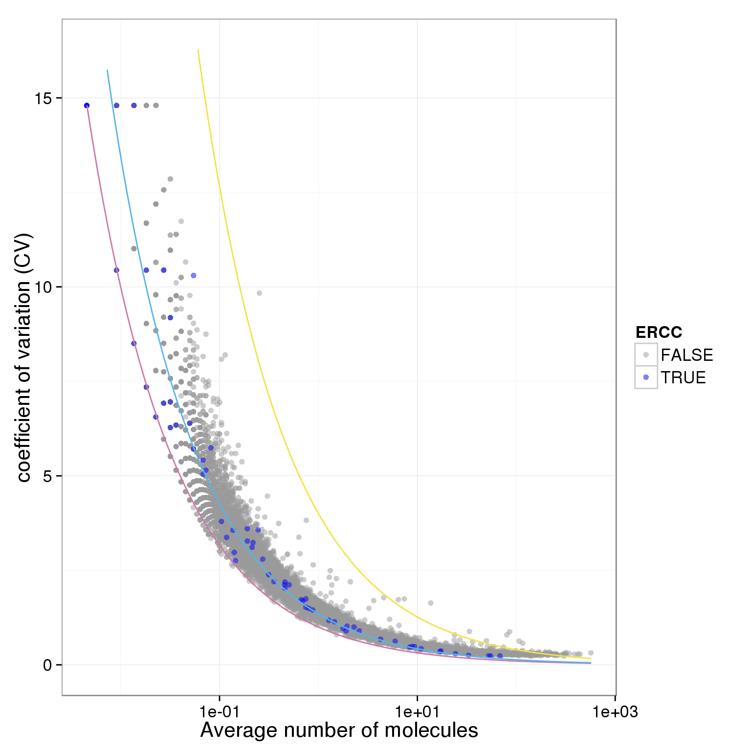
### ignore the following code
 ignore <- function(xxx){
    # log plot
  plot(log(molecules_single_qc_expressed$mean,base=2),log(molecules_single_qc_expressed$CV,base=2), col= "#999999", xlab="log2  Average number of molecules",ylab= "log2 coefficient of variation",ylim=c(-2,5),xlim=c(-10,10),pch=20)
  points(log(molecules_single_qc_expressed_ERCC$mean,base=2),log(molecules_single_qc_expressed_ERCC$CV,base=2),col= "#0000FF" ,pch=20)
  # add lossy poison
  curve(-0.5*x-0.5*log(minipar,base=2),-100,6,add=TRUE,col="#56B4E9")
  # add poisson
  curve(-0.5*x,add=TRUE,col= "#CC79A7")
}
noisy genes
### this function will identify the noisy gene based on 3.7 sd
### only need to specify the input dataset
### the inpute dataset needs to have mean and CV
noisy_gene <- function(data.in){

 #  larger than 4 sd
 count.index  <- (!is.na(data.in$mean))&(data.in$mean>1)
 condi.index <- (data.in$CV > 4*(data.in$mean^(0.5))/data.in$mean)

 sum(count.index&condi.index)

 rownames(molecules_single_qc_expressed)[count.index&condi.index]
}

# noisy genes of all
noisy_gene_all <- noisy_gene(data.in=molecules_single_qc_expressed)

# noisy genes of each individaul
noisy_gene_19098 <- noisy_gene(data.in = individual_19098_mean_CV)
noisy_gene_19101 <- noisy_gene(data.in = individual_19101_mean_CV)
noisy_gene_19239 <- noisy_gene(data.in = individual_19239_mean_CV)
variation between individuals
# overall variation is the sum of inter- and intra- individual variation
# creat a table with all the variation
table_variance <- molecules_single_qc_expressed[,c("gene_name","mean","var","ERCC")]
names(table_variance) <- c("gene_name","mean_all","variance_all","ERCC")

merge_variance <- function(data.base,data.merge,post.name){
  data.merge <- data.merge[,c("gene_name","mean","var")]
  names(data.merge) <- c("gene_name",paste(c("mean","var"),post.name,sep=""))
  merge(data.base,data.merge,by="gene_name",all.x=TRUE)
}
table_variance <- merge_variance(data.base=table_variance,data.merge=individual_19098_mean_CV,post.name="_19098")
table_variance <- merge_variance(data.base=table_variance,data.merge=individual_19101_mean_CV,post.name="_19101")
table_variance <- merge_variance(data.base=table_variance,data.merge=individual_19239_mean_CV,post.name="_19239")

# keep non-missing across the table
table_variance <- table_variance[apply(table_variance,1,function(x)  sum(is.na(x)))==0,]

# number of cell
number.of.cell.all   <- sum(grepl("19",sample_name))
number.of.cell.19098 <- sum(grepl("19098",sample_name))
number.of.cell.19101 <- sum(grepl("19101",sample_name))
number.of.cell.19239 <- sum(grepl("19239",sample_name))

# compute inter individual variance
table_variance$between_indi_var <- (table_variance$variance_all*(number.of.cell.all   -1)  -
 table_variance$var_19098   *(number.of.cell.19098 -1)  -
 table_variance$var_19101   *(number.of.cell.19101 -1)  -
 table_variance$var_19239   *(number.of.cell.19239 -1)  ) /
 (number.of.cell.all -1)

# ratio of inter-individual variance
table_variance$ratio_between_individaul_variance <- table_variance$between_indi_var/table_variance$variance_all

# sellect ERCC
table_variance$ERCC <- grepl("ERCC",table_variance[,1])

# plot ratio of inter-individual variance
ggplot(table_variance, aes(x = variance_all, y = ratio_between_individaul_variance, col = ERCC)) + geom_point(size = 2, alpha = 0.5) + scale_colour_manual(values=cbPalette) + scale_x_log10() + xlab("Variance of all single cell") + ylab("percentage of inter-individual variance") 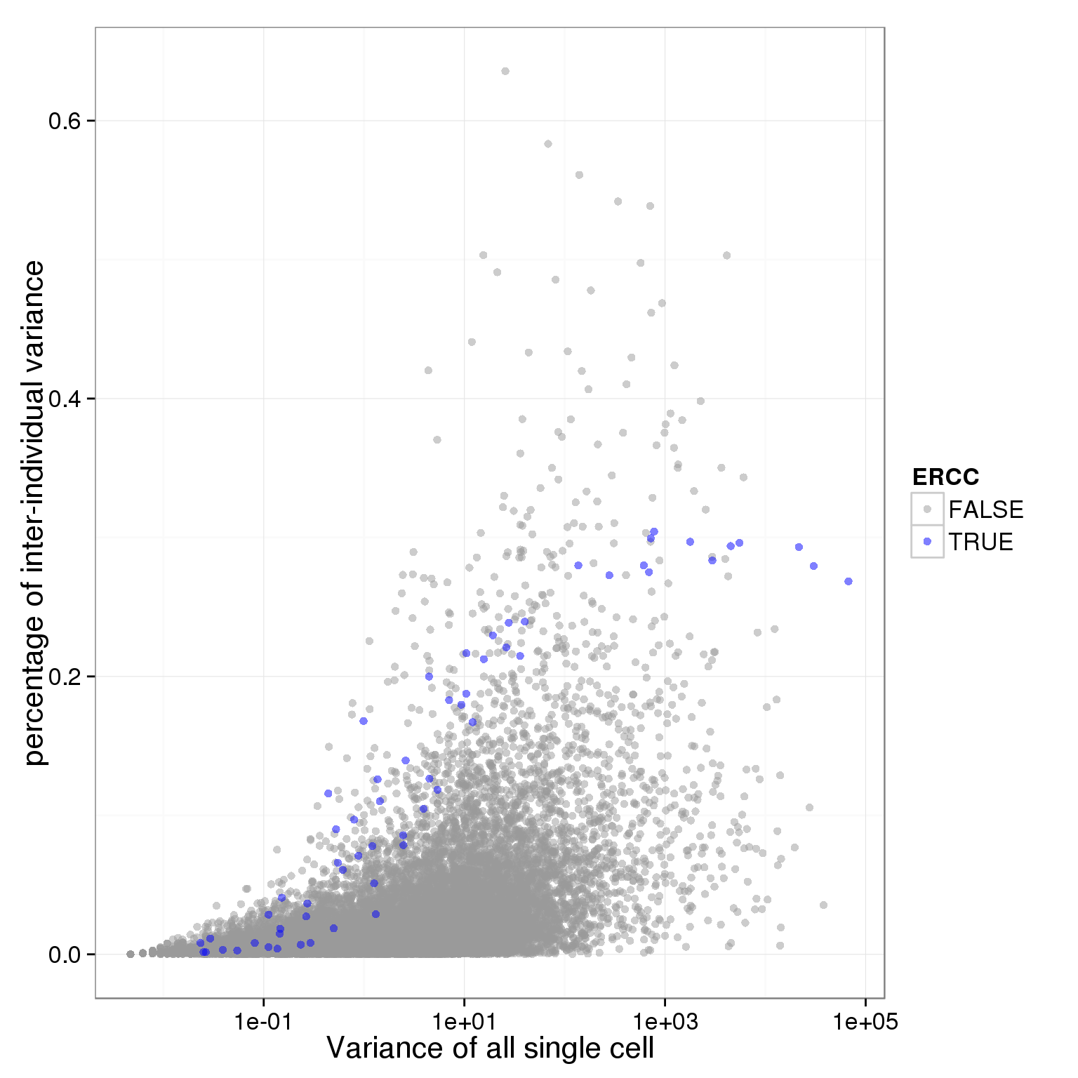
# identify genes that are noisy across all cells and also with a certain level of inter-individual variance
whatever_list <- table_variance[(table_variance$between_indi_var/table_variance$variance_all) > 0.35,][,1]

whatever_list[whatever_list %in% noisy_gene_all]
[1] "ENSG00000069275" "ENSG00000088305" "ENSG00000112306" "ENSG00000117724"
[5] "ENSG00000163041" "ENSG00000166426" "ENSG00000185088" "ENSG00000256618"Session information
sessionInfo()R version 3.2.0 (2015-04-16)
Platform: x86_64-unknown-linux-gnu (64-bit)
locale:
[1] LC_CTYPE=en_US.UTF-8 LC_NUMERIC=C
[3] LC_TIME=en_US.UTF-8 LC_COLLATE=en_US.UTF-8
[5] LC_MONETARY=en_US.UTF-8 LC_MESSAGES=en_US.UTF-8
[7] LC_PAPER=en_US.UTF-8 LC_NAME=C
[9] LC_ADDRESS=C LC_TELEPHONE=C
[11] LC_MEASUREMENT=en_US.UTF-8 LC_IDENTIFICATION=C
attached base packages:
[1] stats graphics grDevices utils datasets methods base
other attached packages:
[1] edgeR_3.10.2 limma_3.24.9 ggplot2_1.0.1 dplyr_0.4.1 knitr_1.10.5
loaded via a namespace (and not attached):
[1] Rcpp_0.11.6 magrittr_1.5 MASS_7.3-40 munsell_0.4.2
[5] colorspace_1.2-6 stringr_1.0.0 plyr_1.8.2 tools_3.2.0
[9] parallel_3.2.0 grid_3.2.0 gtable_0.1.2 DBI_0.3.1
[13] htmltools_0.2.6 lazyeval_0.1.10 yaml_2.1.13 assertthat_0.1
[17] digest_0.6.8 reshape2_1.4.1 formatR_1.2 evaluate_0.7
[21] rmarkdown_0.6.1 labeling_0.3 stringi_0.4-1 scales_0.2.4
[25] proto_0.3-10