Quality control for iPS cells
2015-05-27
Last updated: 2015-10-07
Code version: 5b866c4e43bd9168cd3f4f4621d63daa0d527c49
Input
library("dplyr")
library("ggplot2")
theme_set(theme_bw(base_size = 16))
library("edgeR")
Summary counts from featureCounts. Created with gather-summary-counts.py. These data were collected from the summary files of the full combined samples.
summary_counts <- read.table("../data/summary-counts.txt", header = TRUE,
                             stringsAsFactors = FALSE)
Currently this file only contains data from sickle-trimmed reads, so the code below simply ensures this and then removes the column.
summary_per_sample <- summary_counts %>%
  filter(sickle == "quality-trimmed") %>%
  select(-sickle) %>%
  arrange(individual, batch, well, rmdup) %>%
  as.data.frame
Input annotation.
anno <- read.table("../data/annotation.txt", header = TRUE,
                   stringsAsFactors = FALSE)
head(anno)
individual replicate well batch sample_id
1 NA19098 r1 A01 NA19098.r1 NA19098.r1.A01
2 NA19098 r1 A02 NA19098.r1 NA19098.r1.A02
3 NA19098 r1 A03 NA19098.r1 NA19098.r1.A03
4 NA19098 r1 A04 NA19098.r1 NA19098.r1.A04
5 NA19098 r1 A05 NA19098.r1 NA19098.r1.A05
6 NA19098 r1 A06 NA19098.r1 NA19098.r1.A06Input read counts.
reads <- read.table("../data/reads.txt", header = TRUE,
                    stringsAsFactors = FALSE)
Input molecule counts.
molecules <- read.table("../data/molecules.txt", header = TRUE,
                    stringsAsFactors = FALSE)
Input single cell observational quality control data.
qc <- read.table("../data/qc-ipsc.txt", header = TRUE,
                 stringsAsFactors = FALSE)
head(qc)
individual batch well cell_number concentration tra1.60
1 19098 1 A01 1 1.734785 1
2 19098 1 A02 1 1.723038 1
3 19098 1 A03 1 1.512786 1
4 19098 1 A04 1 1.347492 1
5 19098 1 A05 1 2.313047 1
6 19098 1 A06 1 2.056803 1Total mapped reads, unmapped ratios, and ERCC ratios
Looking at the unmapped ratio and ERCC ratio of each cell based on number of reads.
- low number of mapped reads might be caused by cell apoptosis, RNA degradation, insufficient cell lysis, bad Tn5 transposase quality, or contamination
- high proportion of ERCC spike-in indicates low RNA quantity from iPSCs which might cell death
# reads per sample
summary_per_sample_reads <- summary_per_sample %>% filter(rmdup == "reads")

# create unmapped ratios
summary_per_sample_reads$unmapped.ratios <- summary_per_sample_reads[,9]/apply(summary_per_sample_reads[,5:13],1,sum)

# create total mapped reads
summary_per_sample_reads$total.mapped <- apply(summary_per_sample_reads[,5:8],1,sum)

# plot
ggplot(summary_per_sample_reads, aes(x = total.mapped, y = unmapped.ratios, col = as.factor(individual), shape = as.factor(batch))) + geom_point(size = 3, alpha = 0.5)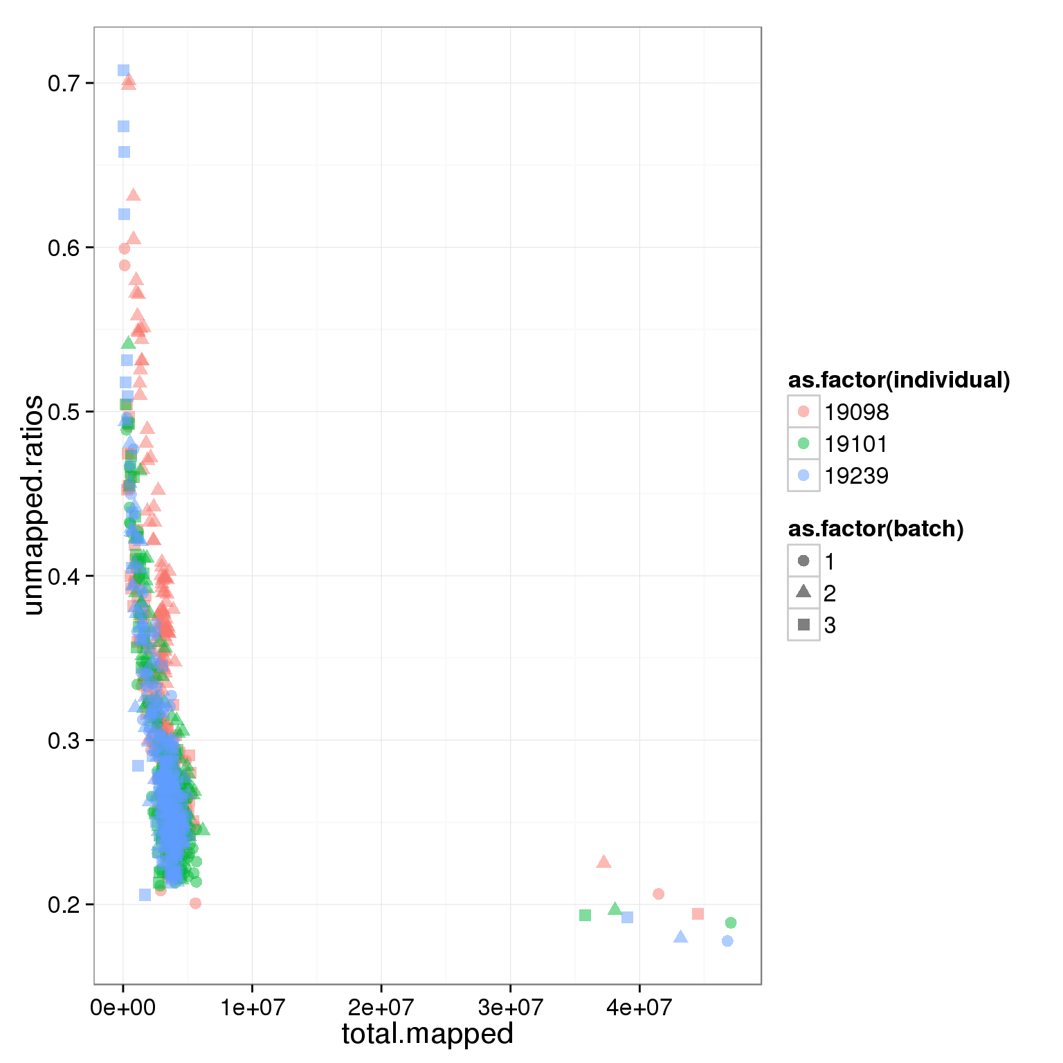
Looking at only the single cell libraries
# remove bulk keep single cell
summary_per_sample_reads_single <- summary_per_sample_reads[summary_per_sample_reads$well!="bulk",]

# total ERCC reads
summary_per_sample_reads_single$total.ERCC <- apply(reads[grep("ERCC", rownames(reads)), ],2,sum)
plot(summary_per_sample_reads_single$total.ERCC)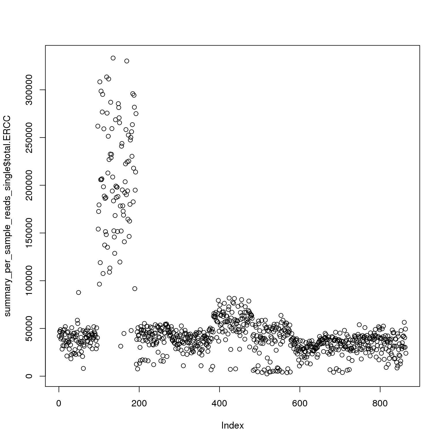
# creat ERCC ratios
summary_per_sample_reads_single$ERCC.ratios <- apply(reads[grep("ERCC", rownames(reads)), ],2,sum)/apply(summary_per_sample_reads_single[,5:8],1,sum)

# many plots
ggplot(summary_per_sample_reads_single, aes(x = total.mapped, y = unmapped.ratios, col = as.factor(individual), shape = as.factor(batch))) + geom_point(size = 3, alpha = 0.5) + xlab("Number of mapped reads") + ylab("Umapped reads ratio")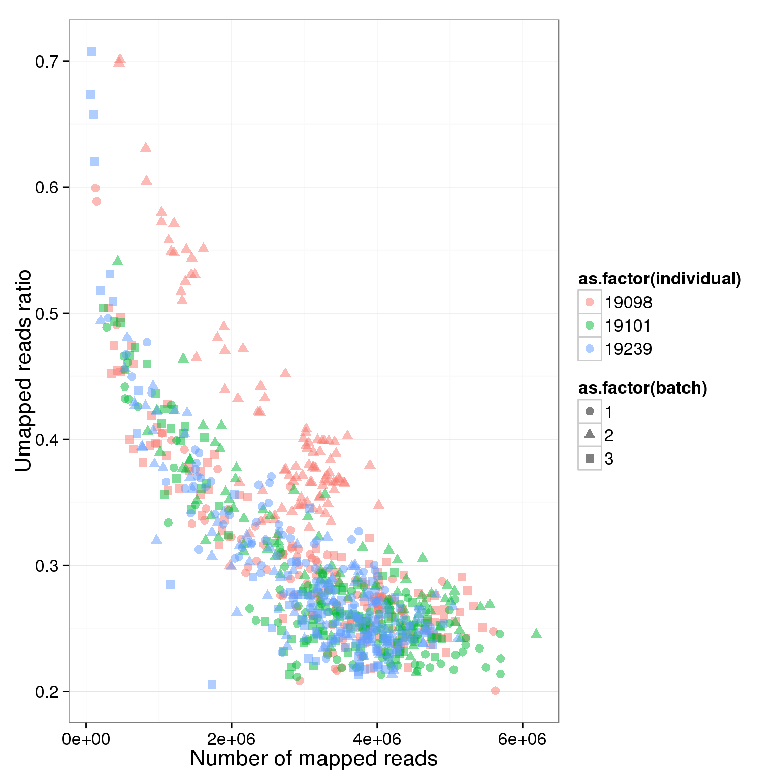
ggplot(summary_per_sample_reads_single, aes(x = total.mapped, y = ERCC.ratios, col = as.factor(individual), shape = as.factor(batch))) + geom_point(size = 3, alpha = 0.5) + xlab("Number of mapped reads") + ylab("Spike-in reads ratio")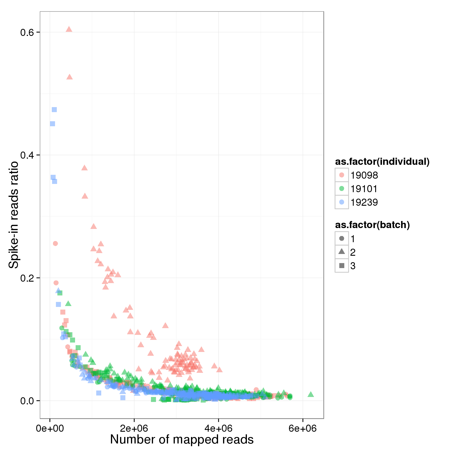
ggplot(summary_per_sample_reads_single, aes(x = total.mapped, y = unmapped.ratios, col = as.factor(individual), shape = as.factor(batch))) + geom_point(size = 3, alpha = 0.5) + facet_grid(individual ~ batch) + theme(axis.text.x = element_text(angle = 90, hjust = 0.9, vjust = 0.5))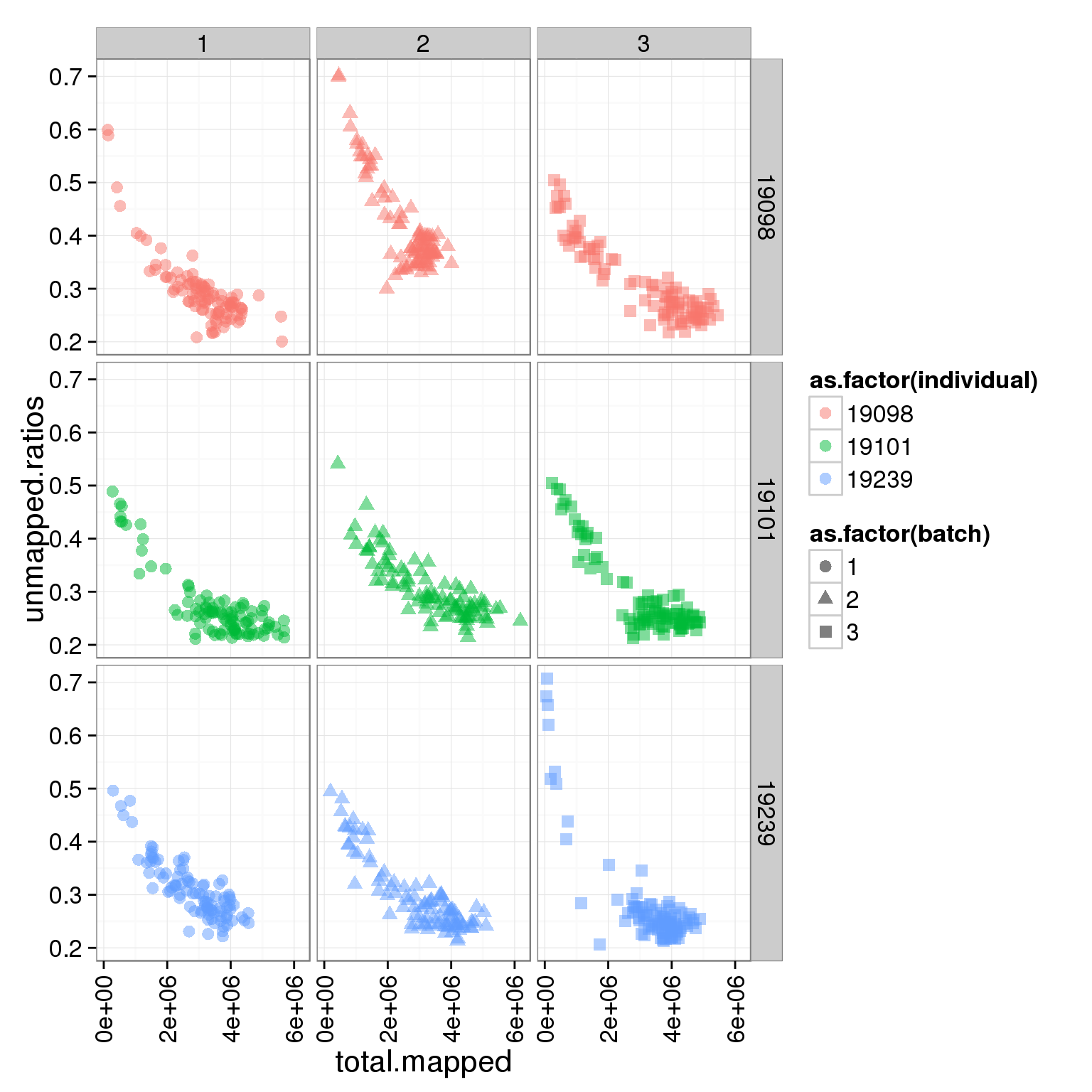
ggplot(summary_per_sample_reads_single, aes(x = total.mapped, y = ERCC.ratios, col = as.factor(individual), shape = as.factor(batch))) + geom_point(size = 3, alpha = 0.5) + facet_grid(individual ~ batch) + theme(axis.text.x = element_text(angle = 90, hjust = 0.9, vjust = 0.5))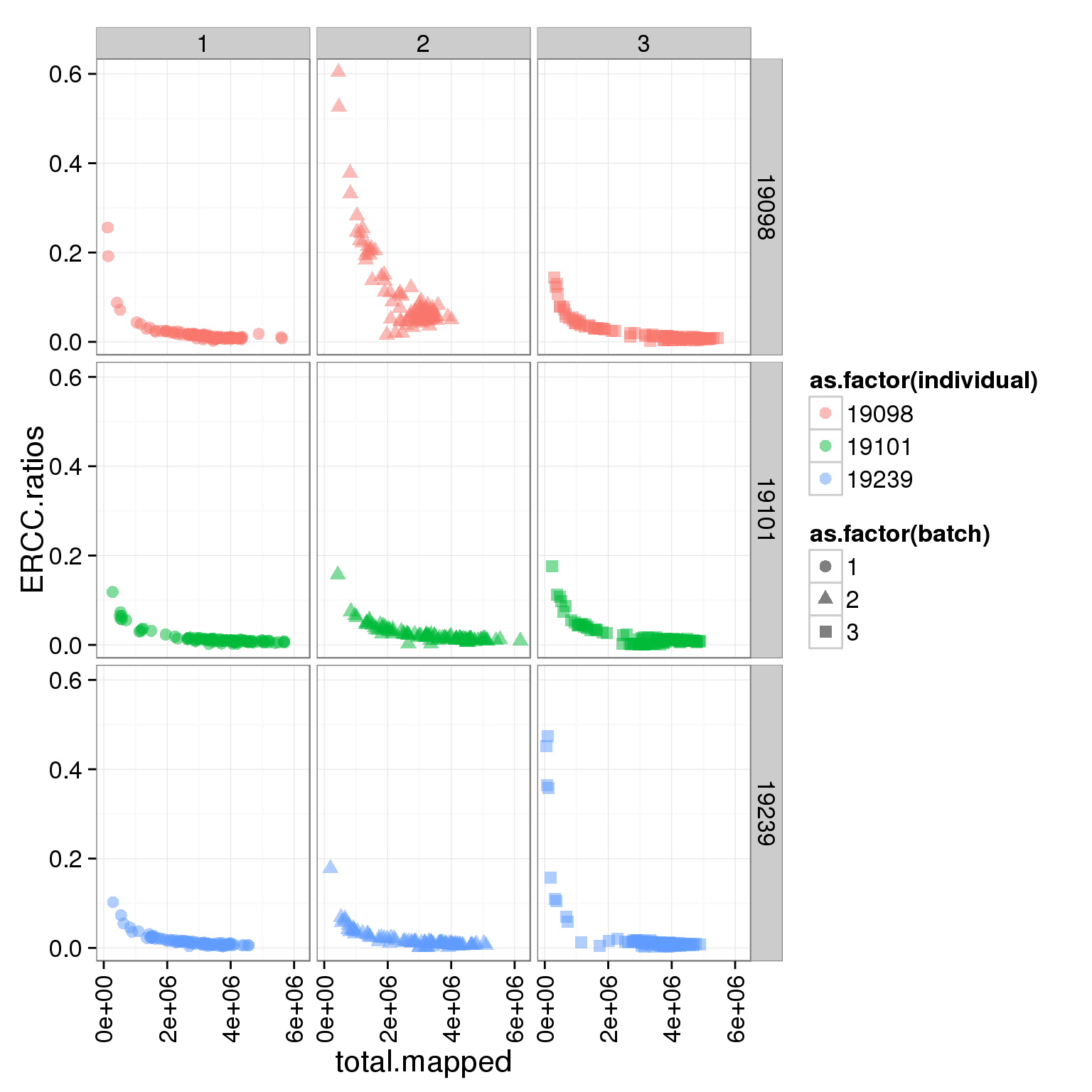
ggplot(summary_per_sample_reads_single, aes(x = total.mapped, y = total.ERCC, col = as.factor(individual), shape = as.factor(batch))) + geom_point(size = 3, alpha = 0.5) + facet_grid(individual ~ batch) + theme(axis.text.x = element_text(angle = 90, hjust = 0.9, vjust = 0.5))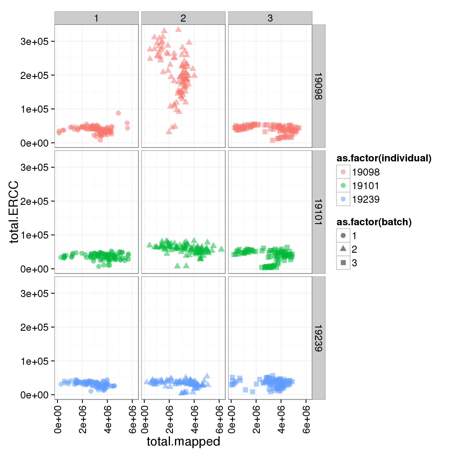
Total molecules of ERCC and endogenous genes
Looking at the total molecule number of ERCC and endogenous genes
summary_per_sample_reads_single$total_ERCC_molecule <- apply(molecules[grep("ERCC", rownames(molecules)), ],2,sum)

summary_per_sample_reads_single$total_gene_molecule <- apply(molecules[grep("ENSG", rownames(molecules)), ],2,sum)

ggplot(summary_per_sample_reads_single, aes(x = total.mapped, y = total_gene_molecule, col = as.factor(individual), shape = as.factor(batch), label = well)) + geom_point(size = 3, alpha = 0.5) + xlab("Total mapped reads") + ylab("Total gene molecule")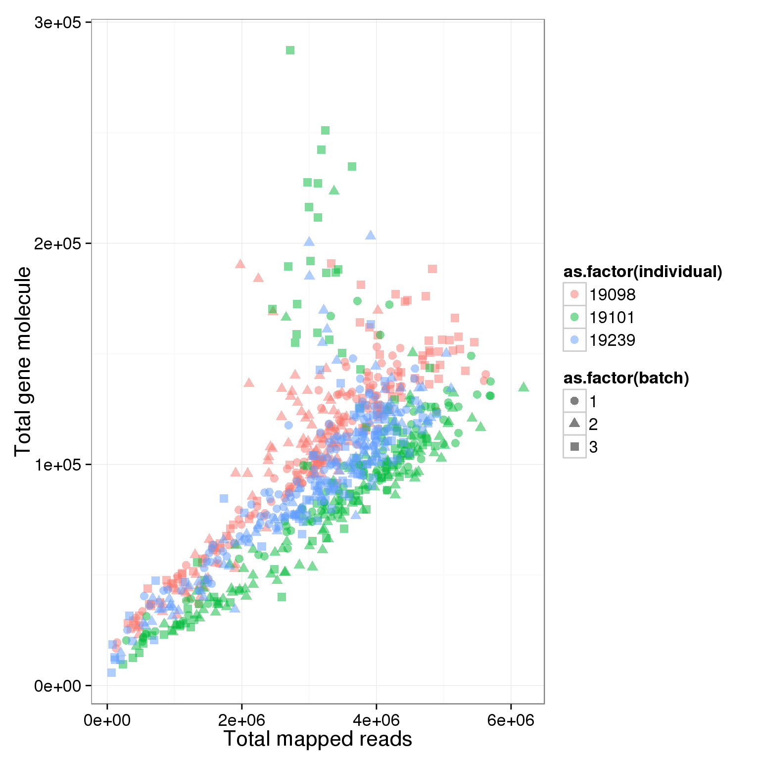
total_ERCC_plot <- ggplot(summary_per_sample_reads_single, aes(x = total.mapped, y = total_ERCC_molecule, col = as.factor(individual), shape = as.factor(batch), label = well)) + geom_point(size = 3, alpha = 0.5) + xlab("Total mapped reads") + ylab("Total ERCC molecule")

total_ERCC_plot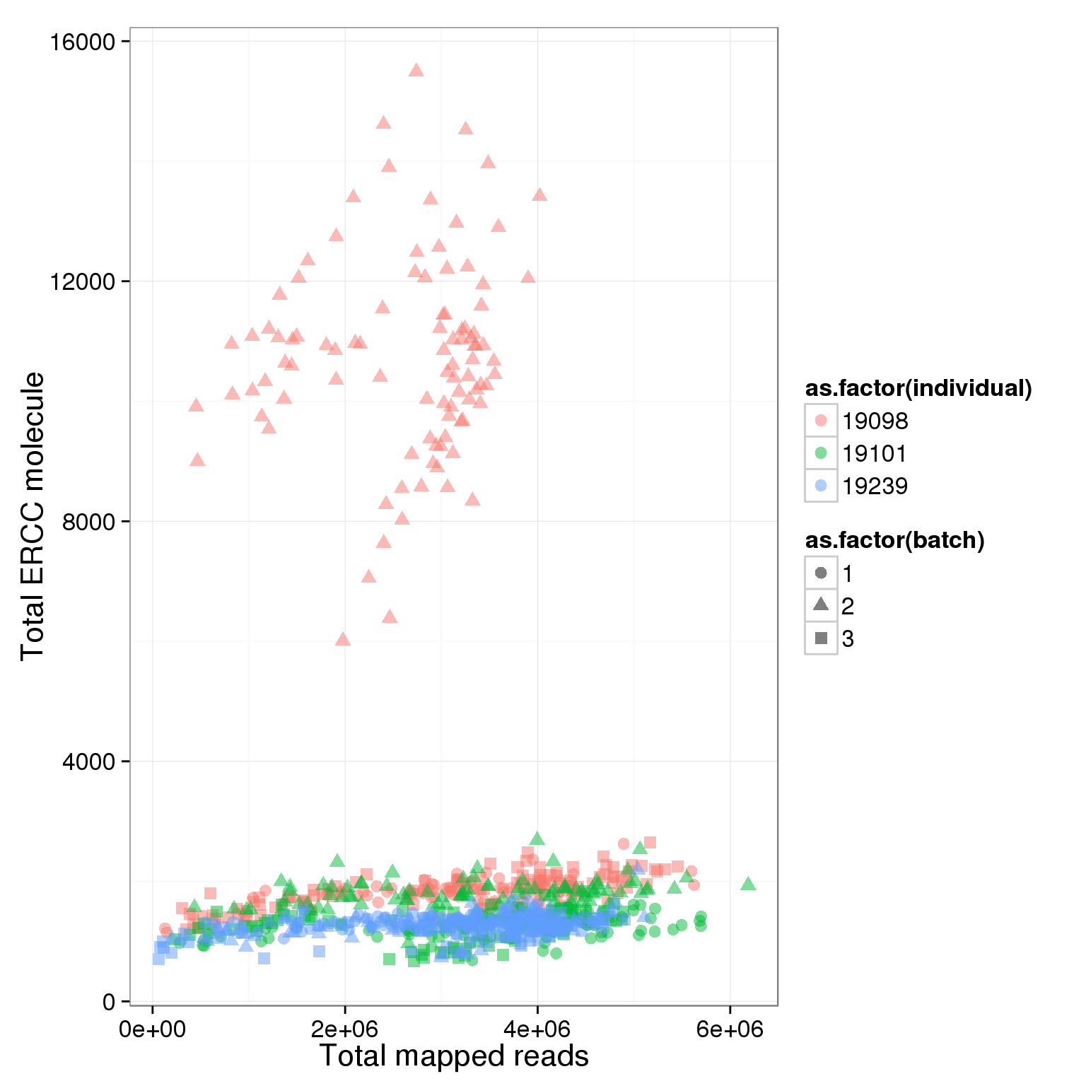
total_ERCC_plot + facet_grid(individual ~ batch) + geom_smooth()geom_smooth: method="auto" and size of largest group is <1000, so using loess. Use 'method = x' to change the smoothing method.
geom_smooth: method="auto" and size of largest group is <1000, so using loess. Use 'method = x' to change the smoothing method.
geom_smooth: method="auto" and size of largest group is <1000, so using loess. Use 'method = x' to change the smoothing method.
geom_smooth: method="auto" and size of largest group is <1000, so using loess. Use 'method = x' to change the smoothing method.
geom_smooth: method="auto" and size of largest group is <1000, so using loess. Use 'method = x' to change the smoothing method.
geom_smooth: method="auto" and size of largest group is <1000, so using loess. Use 'method = x' to change the smoothing method.
geom_smooth: method="auto" and size of largest group is <1000, so using loess. Use 'method = x' to change the smoothing method.
geom_smooth: method="auto" and size of largest group is <1000, so using loess. Use 'method = x' to change the smoothing method.
geom_smooth: method="auto" and size of largest group is <1000, so using loess. Use 'method = x' to change the smoothing method.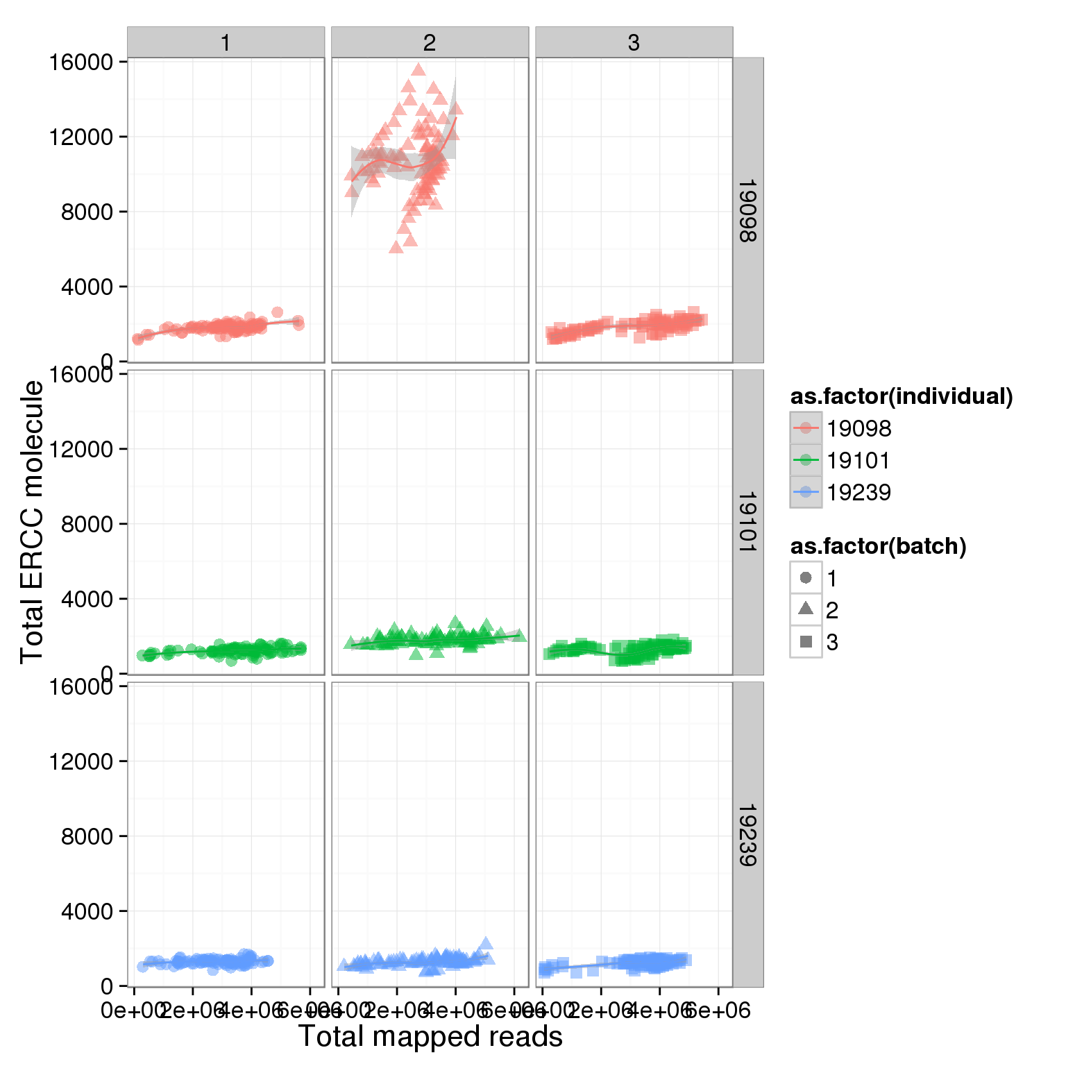
total_ERCC_plot + scale_y_continuous(limits=c(0, 4000)) + facet_grid(individual ~ batch) + geom_smooth()geom_smooth: method="auto" and size of largest group is <1000, so using loess. Use 'method = x' to change the smoothing method.
geom_smooth: method="auto" and size of largest group is <1000, so using loess. Use 'method = x' to change the smoothing method.Warning: Removed 96 rows containing missing values (stat_smooth).geom_smooth: method="auto" and size of largest group is <1000, so using loess. Use 'method = x' to change the smoothing method.
geom_smooth: method="auto" and size of largest group is <1000, so using loess. Use 'method = x' to change the smoothing method.
geom_smooth: method="auto" and size of largest group is <1000, so using loess. Use 'method = x' to change the smoothing method.
geom_smooth: method="auto" and size of largest group is <1000, so using loess. Use 'method = x' to change the smoothing method.
geom_smooth: method="auto" and size of largest group is <1000, so using loess. Use 'method = x' to change the smoothing method.
geom_smooth: method="auto" and size of largest group is <1000, so using loess. Use 'method = x' to change the smoothing method.
geom_smooth: method="auto" and size of largest group is <1000, so using loess. Use 'method = x' to change the smoothing method.Warning: Removed 96 rows containing missing values (geom_point).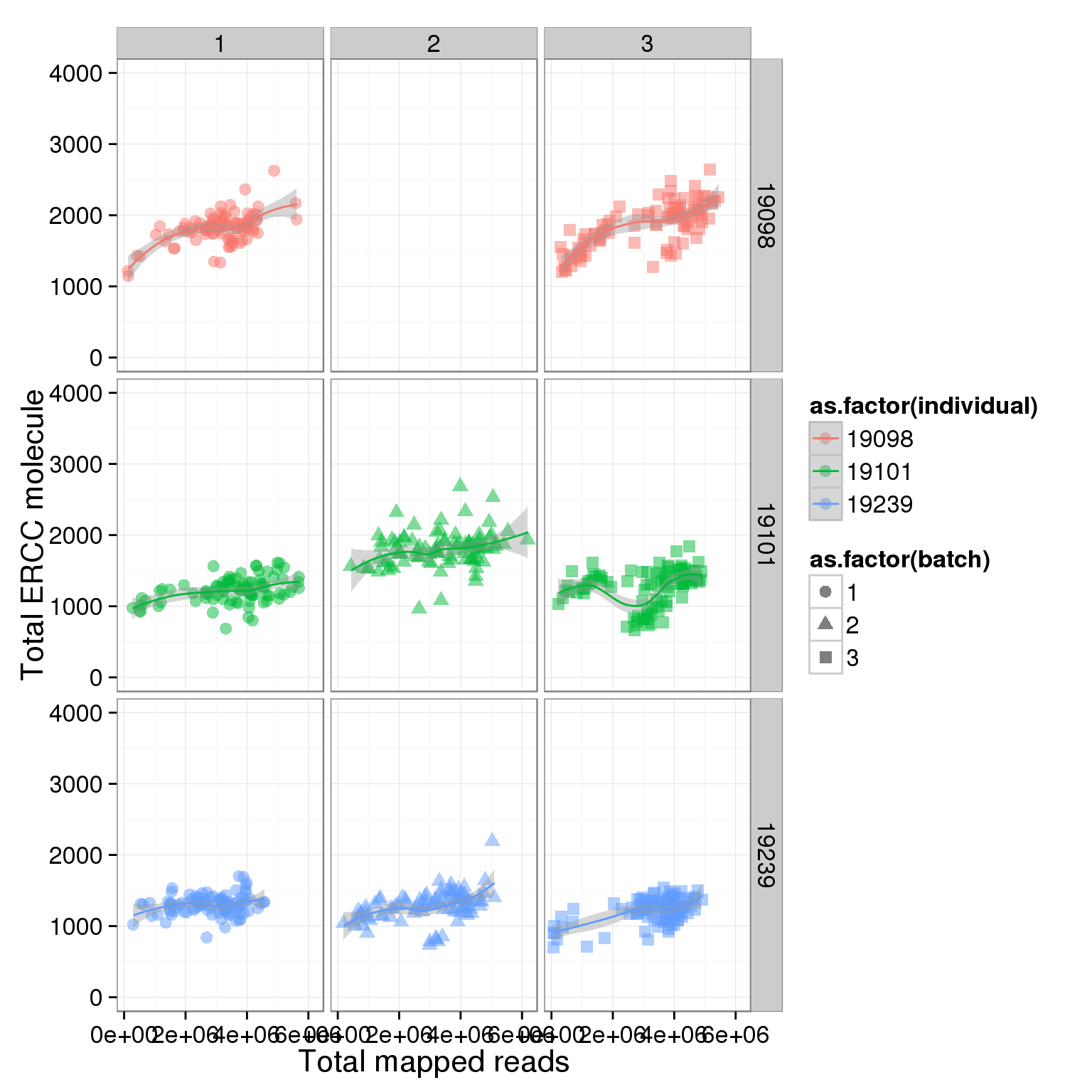
plot(summary_per_sample_reads_single$total_ERCC_molecule)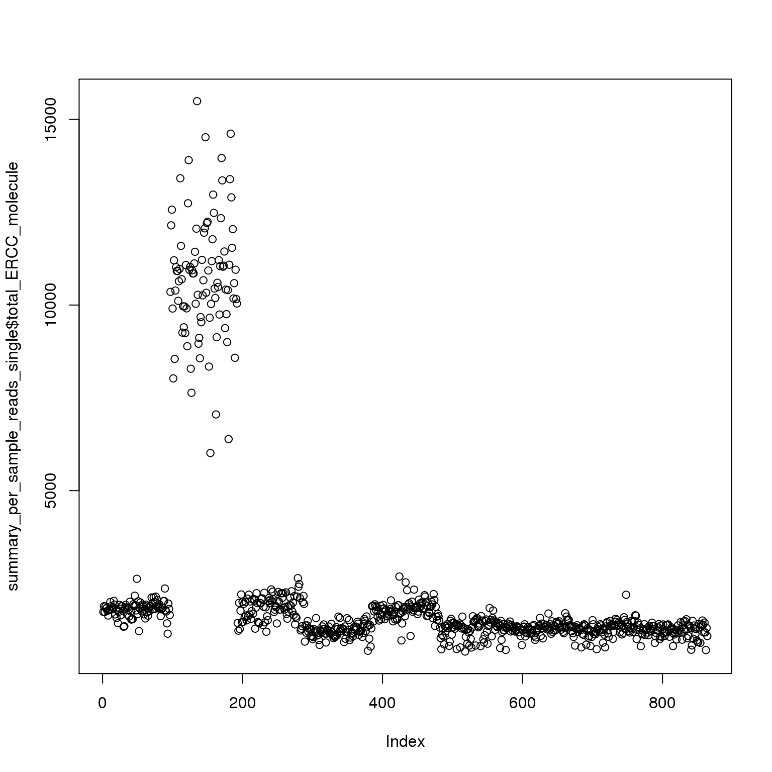
Adjust the ERCC total reads of 19098 batch 2
It is obvious that the 19098 batch 2 have a lot more ERCC than all the other. Here is trying to fix it by adjusting the ERCC of the super sad batch.
summary_per_sample_reads_single$index_19098_2 <- (summary_per_sample_reads_single$individual=="19098" & summary_per_sample_reads_single$batch=="2")

#calculating the ratio of 19098 batch 2 to the rest
adjusted_ratio <- mean(summary_per_sample_reads_single$total.ERCC[summary_per_sample_reads_single$index_19098_2])/mean(summary_per_sample_reads_single$total.ERCC[!summary_per_sample_reads_single$index_19098_2])

adjusted_ratio
[1] 5.315369#adjusted total ERCC reads
summary_per_sample_reads_single$adj.total.ERCC <- summary_per_sample_reads_single$total.ERCC
summary_per_sample_reads_single$adj.total.ERCC[summary_per_sample_reads_single$index_19098_2] <- summary_per_sample_reads_single$adj.total.ERCC[summary_per_sample_reads_single$index_19098_2]/adjusted_ratio
#adjust ERCC ratio
summary_per_sample_reads_single$adj.ERCC.ratios <-
summary_per_sample_reads_single$adj.total.ERCC/summary_per_sample_reads_single$total.mapped
ggplot(summary_per_sample_reads_single, aes(x = total.mapped, y = adj.ERCC.ratios, col = as.factor(individual), shape = as.factor(batch))) + geom_point(size = 3, alpha = 0.5) + facet_grid(individual ~ batch) + theme(axis.text.x = element_text(angle = 90, hjust = 0.9, vjust = 0.5))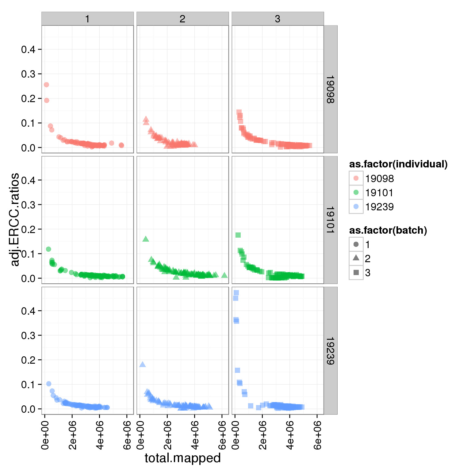
Cell number
The cell number of each capture site is recorded after the cell corting step and before the cells got lysed.
#add cell number per well by merging qc file
summary_per_sample_reads_single_qc <- merge(summary_per_sample_reads_single,qc,by=c("individual","batch","well"))

ggplot(summary_per_sample_reads_single_qc, aes(x = total.mapped, y = unmapped.ratios, col = as.factor(individual), label = as.character(cell_number))) + geom_text(fontface=3)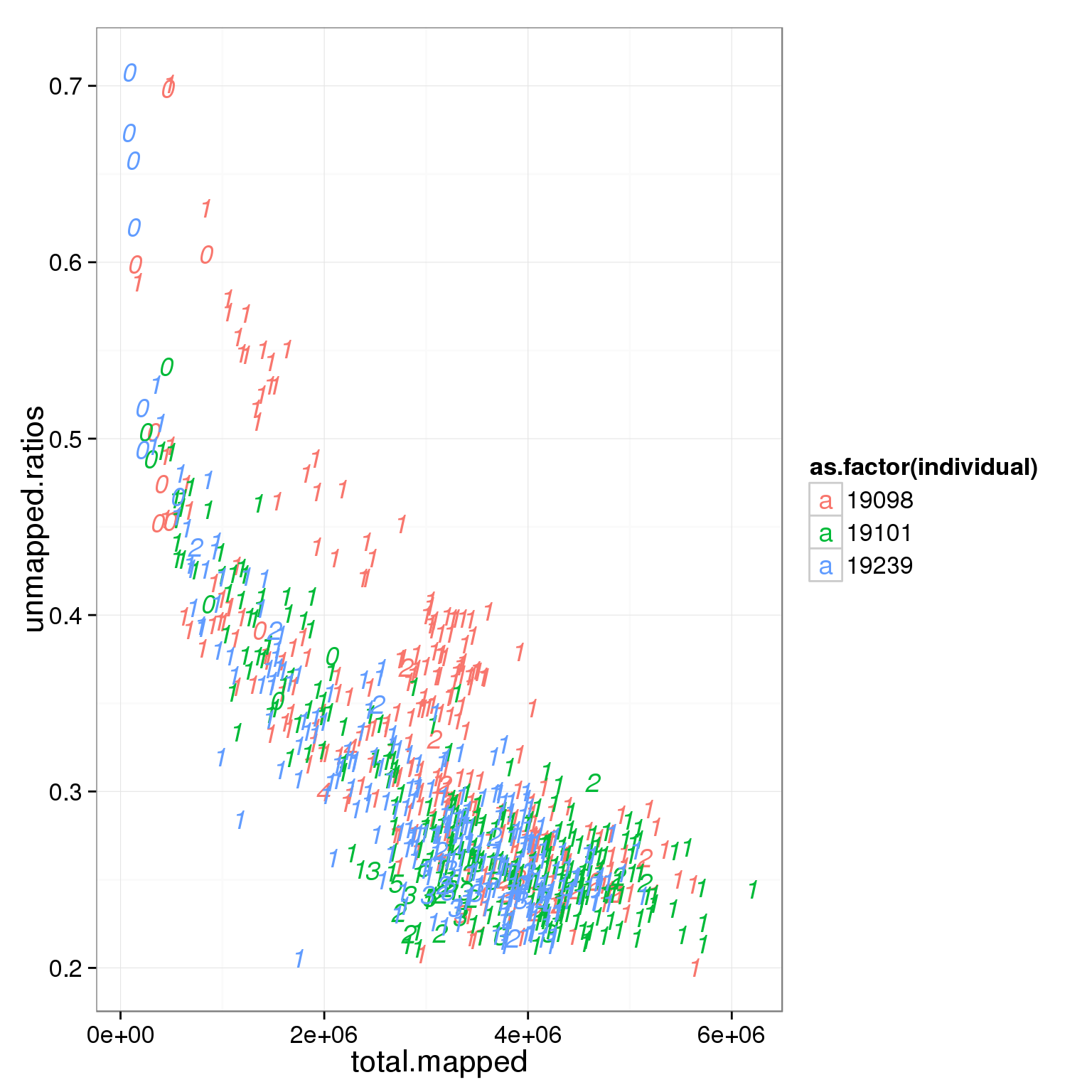
ggplot(summary_per_sample_reads_single_qc, aes(x = total.mapped, y = ERCC.ratios, col = as.factor(individual), label = as.character(cell_number))) + geom_text(fontface=3)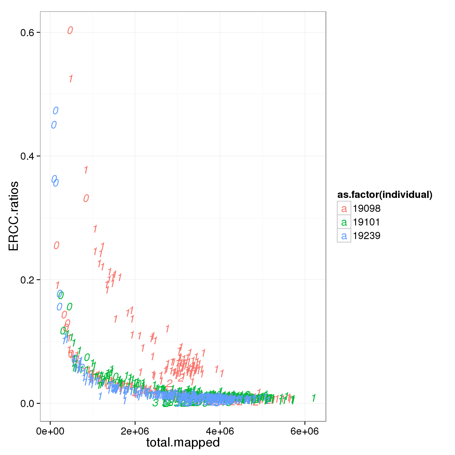
# look at total molecule
ggplot(summary_per_sample_reads_single_qc, aes(x = total.mapped, y = total_gene_molecule, col = as.factor(individual), label = as.character(cell_number))) + xlab("Total mapped reads") + ylab("Total endogenous gene molecule") + geom_text(fontface=3)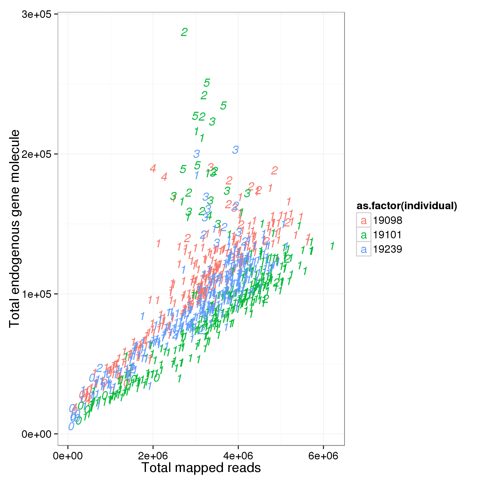
Based on the observation that these is a dinstint cell population with more than 1.5 million reads, we used it as a cutoff.
#qc filter only keep cells with more than 1.5 million reads
summary_per_sample_reads_single_qc$qc_filter <- summary_per_sample_reads_single_qc$cell_number == 1 & summary_per_sample_reads_single_qc$total.mapped > 1.5 * 10^6

ggplot(summary_per_sample_reads_single_qc, aes(x = total.mapped, y = unmapped.ratios, col = qc_filter, label = as.character(cell_number))) + geom_text(fontface=3) + facet_grid(individual ~ batch) + theme(axis.text.x = element_text(angle = 90, hjust = 0.9, vjust = 0.5)) + xlab("Number of mapped reads") + ylab("Umapped reads ratio")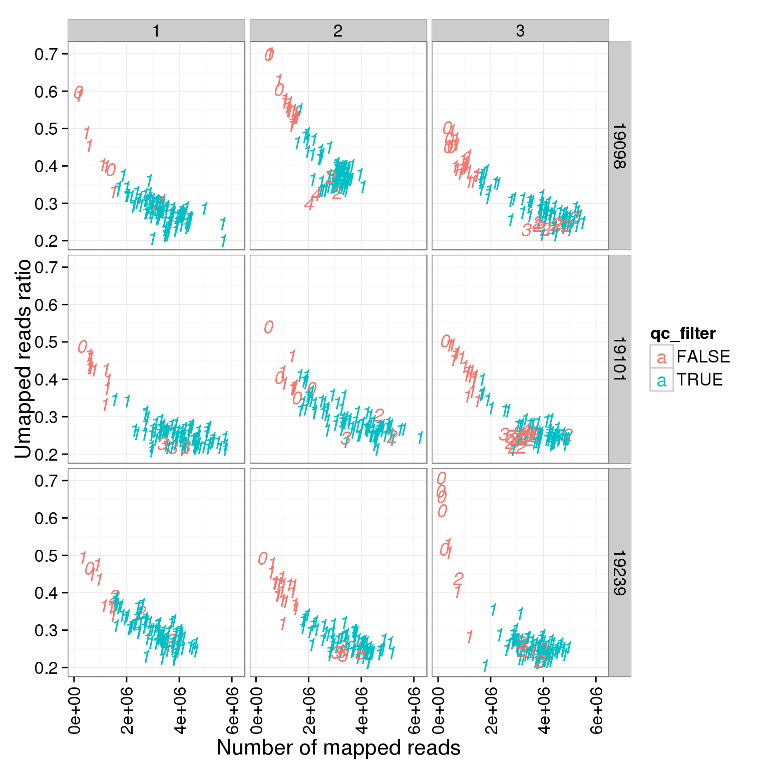
ggplot(summary_per_sample_reads_single_qc, aes(x = total.mapped, y = ERCC.ratios, col = qc_filter, label = as.character(cell_number))) + geom_text(fontface=3) + facet_grid(individual ~ batch) + theme(axis.text.x = element_text(angle = 90, hjust = 0.9, vjust = 0.5)) + xlab("Number of mapped reads") + ylab("Spike-in reads ratio")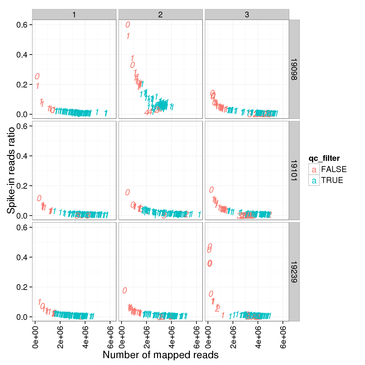
Number of genes detected
## number of expressed gene in each cell
reads_single <- reads
reads_single_gene_number <- colSums(reads_single > 1)
summary_per_sample_reads_single_qc$reads_single_gene_number <- reads_single_gene_number

ggplot(summary_per_sample_reads_single_qc, aes(x = total.mapped, y = reads_single_gene_number, col = qc_filter, label = as.character(cell_number))) + geom_text(fontface=3) + facet_grid(individual ~ batch) + theme(axis.text.x = element_text(angle = 90, hjust = 0.9, vjust = 0.5)) + xlab("Number of mapped reads") + ylab("Number of genes")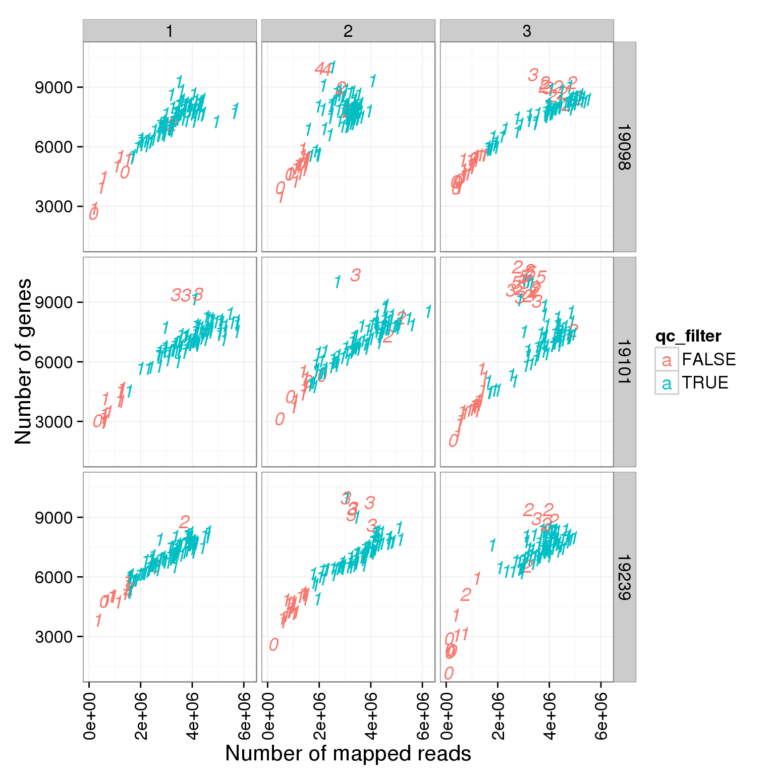
ggplot(summary_per_sample_reads_single_qc, aes(x = reads_single_gene_number, y = ERCC.ratios, col = qc_filter, label = as.character(cell_number))) + geom_text(fontface=3) + facet_grid(individual ~ batch) + theme(axis.text.x = element_text(angle = 90, hjust = 0.9, vjust = 0.5)) + xlab("Number of genes") + ylab("Spike-in reads ratio")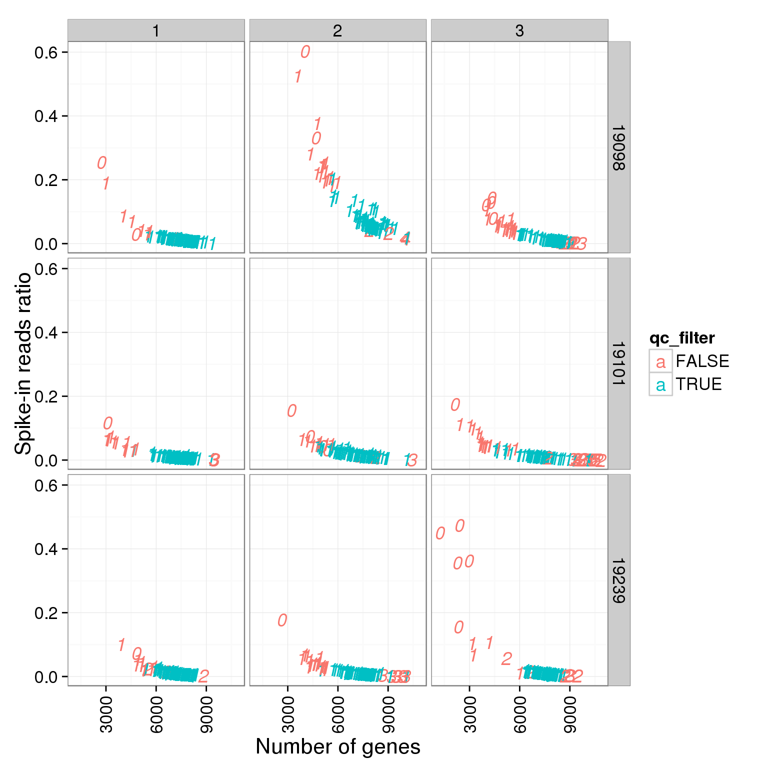
Reads mapped to mitochondrial genes
## create a list of mitochondrial genes (13 protein-coding genes)
## MT-ATP6, MT-CYB, MT-ND1, MT-ND4, MT-ND4L, MT-ND5, MT-ND6, MT-CO2, MT-CO1, MT-ND2, MT-ATP8, MT-CO3, MT-ND3
mtgene <- c("ENSG00000198899", "ENSG00000198727", "ENSG00000198888", "ENSG00000198886", "ENSG00000212907", "ENSG00000198786", "ENSG00000198695", "ENSG00000198712", "ENSG00000198804", "ENSG00000198763","ENSG00000228253", "ENSG00000198938", "ENSG00000198840")

## reads of mt genes in single cells
mt_reads <- reads_single[mtgene,]
dim(mt_reads)
[1] 13 864## mt ratio of single cell
mt_reads_total <- apply(mt_reads, 2, sum)
summary_per_sample_reads_single_qc$mt_reads_total <- mt_reads_total
summary_per_sample_reads_single_qc$mt_reads_ratio <- summary_per_sample_reads_single_qc$mt_reads_total/summary_per_sample_reads_single_qc$total.mapped
ggplot(summary_per_sample_reads_single_qc, aes(x = total.mapped, y = mt_reads_ratio, col = qc_filter, label = as.character(cell_number))) + geom_text(fontface=3) + facet_grid(individual ~ batch) + theme(axis.text.x = element_text(angle = 90, hjust = 0.9, vjust = 0.5)) + xlab("Number of mapped reads") + ylab("Mitochondrial ratio")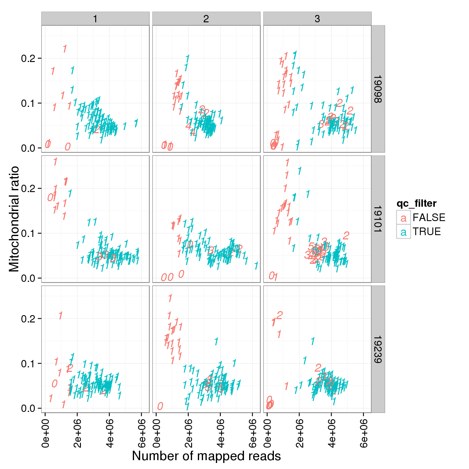
ggplot(summary_per_sample_reads_single_qc, aes(x = mt_reads_ratio, y = ERCC.ratios, col = qc_filter, label = as.character(cell_number))) + geom_text(fontface=3) + facet_grid(individual ~ batch) + theme(axis.text.x = element_text(angle = 90, hjust = 0.9, vjust = 0.5)) + xlab("Mitochondrial ratio") + ylab("Spike-in reads ratio")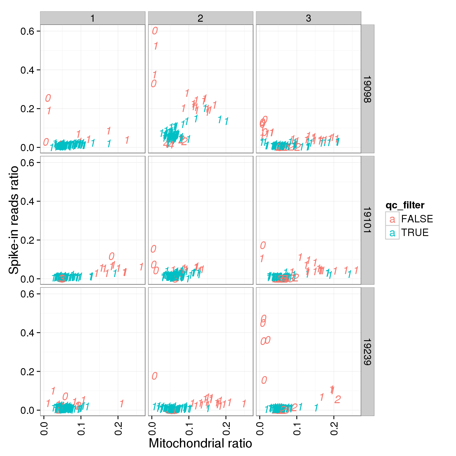
ggplot(summary_per_sample_reads_single_qc, aes(x = reads_single_gene_number, y = mt_reads_ratio, col = qc_filter, label = as.character(cell_number))) + geom_text(fontface=3) + facet_grid(individual ~ batch) + theme(axis.text.x = element_text(angle = 90, hjust = 0.9, vjust = 0.5)) + xlab("Number of genes") + ylab("Mitochondrial ratio")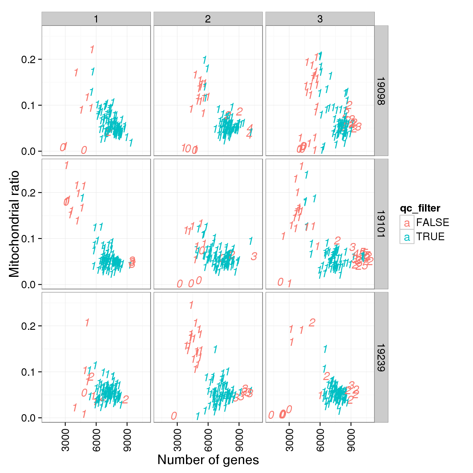
Effect of cell QC data on sequencing results
Cell number
table(summary_per_sample_reads_single_qc$cell_number)
  0   1   2   3   4   5
 21 789  29  17   3   5
ggplot(summary_per_sample_reads_single_qc,
aes(x = as.factor(cell_number), y = ERCC.ratios)) +
geom_boxplot()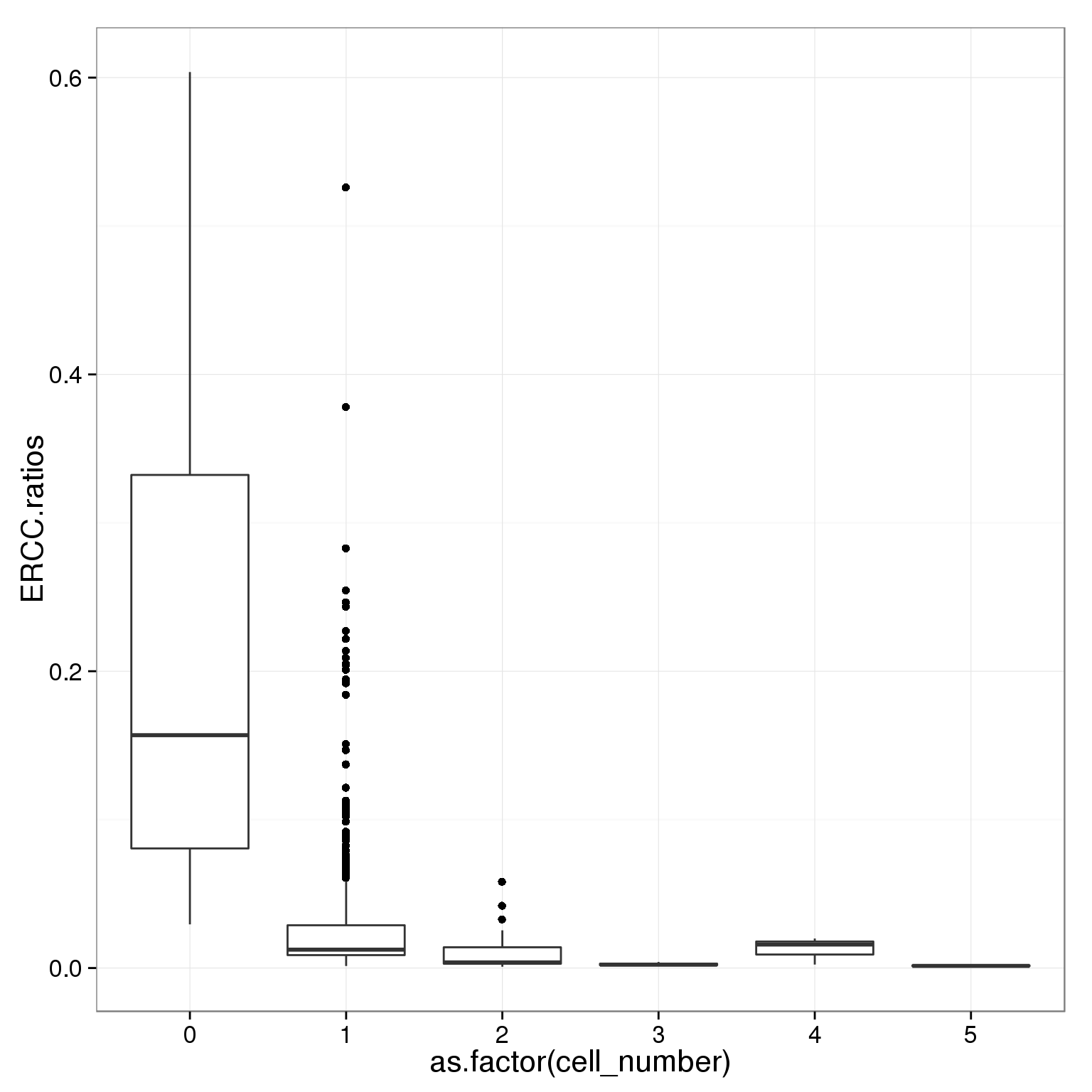
ggplot(summary_per_sample_reads_single_qc,
       aes(x = as.factor(cell_number), y = unmapped.ratios)) +
  geom_boxplot()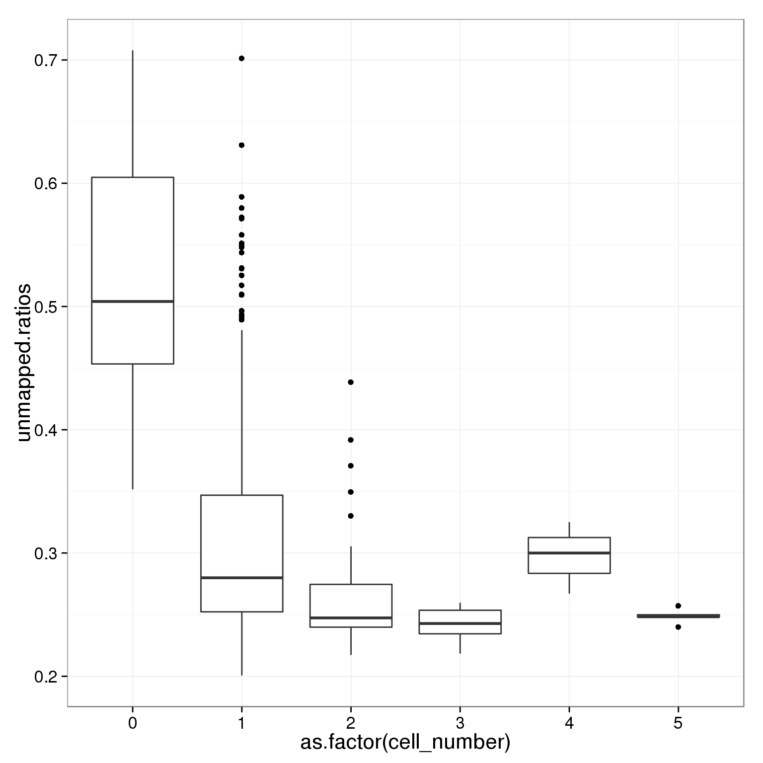
Concentration
summary(summary_per_sample_reads_single_qc$concentration) Min. 1st Qu. Median Mean 3rd Qu. Max.
0.000 1.030 1.680 1.545 2.081 3.200 ggplot(summary_per_sample_reads_single_qc,
aes(x = concentration, y = ERCC.ratios)) +
geom_point() +
geom_smooth()geom_smooth: method="auto" and size of largest group is <1000, so using loess. Use 'method = x' to change the smoothing method.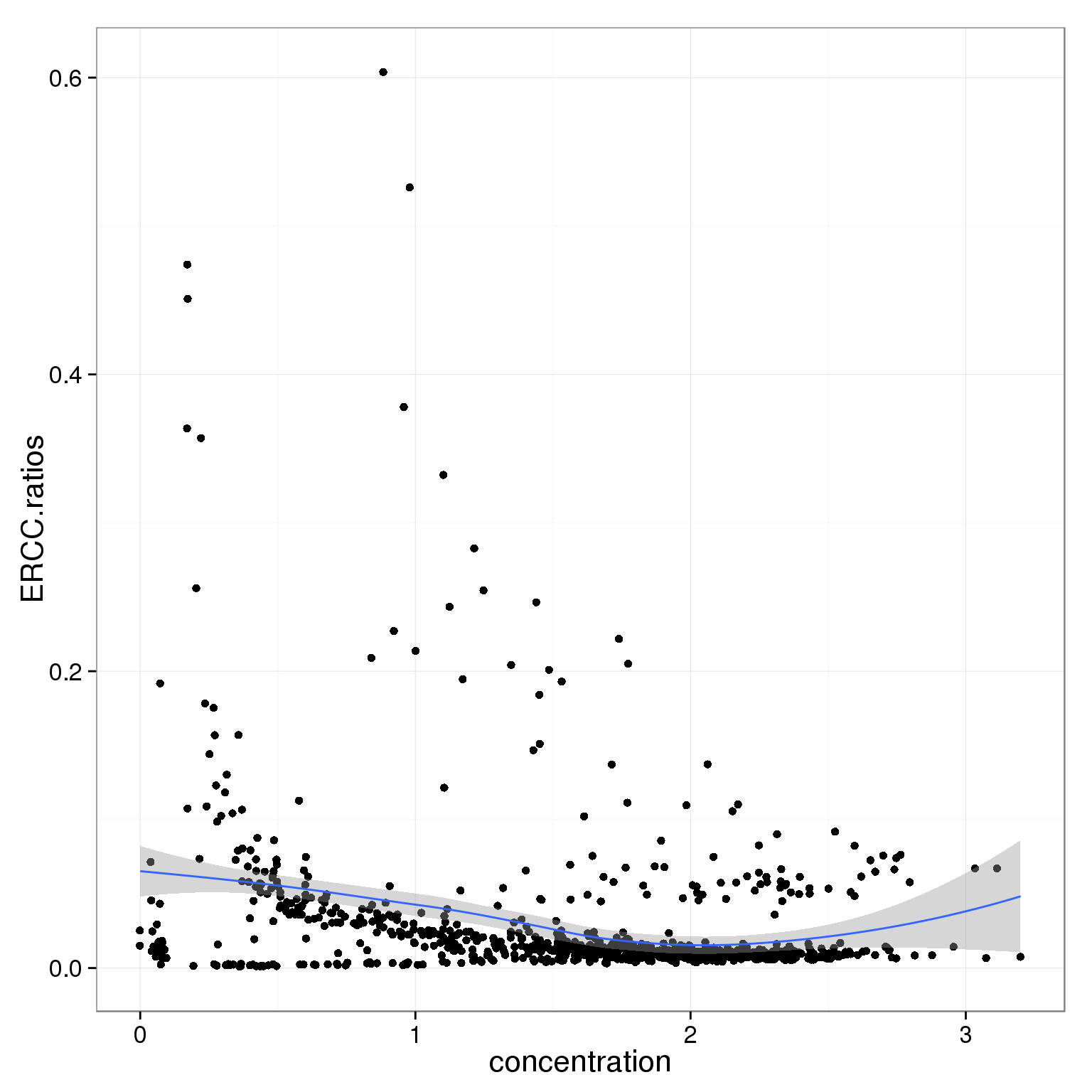
ggplot(summary_per_sample_reads_single_qc,
       aes(x = concentration, y = unmapped.ratios)) +
  geom_point() +
  geom_smooth()
geom_smooth: method="auto" and size of largest group is <1000, so using loess. Use 'method = x' to change the smoothing method.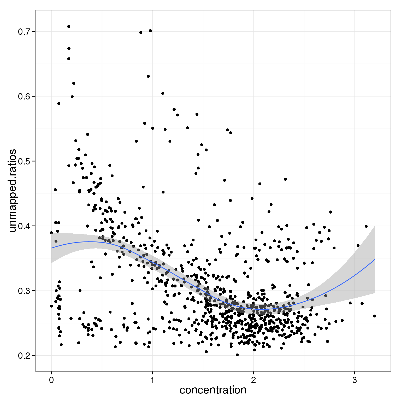
ggplot(summary_per_sample_reads_single_qc,
       aes(x = concentration, y = total.mapped)) +
  geom_point() +
  geom_smooth()
geom_smooth: method="auto" and size of largest group is <1000, so using loess. Use 'method = x' to change the smoothing method.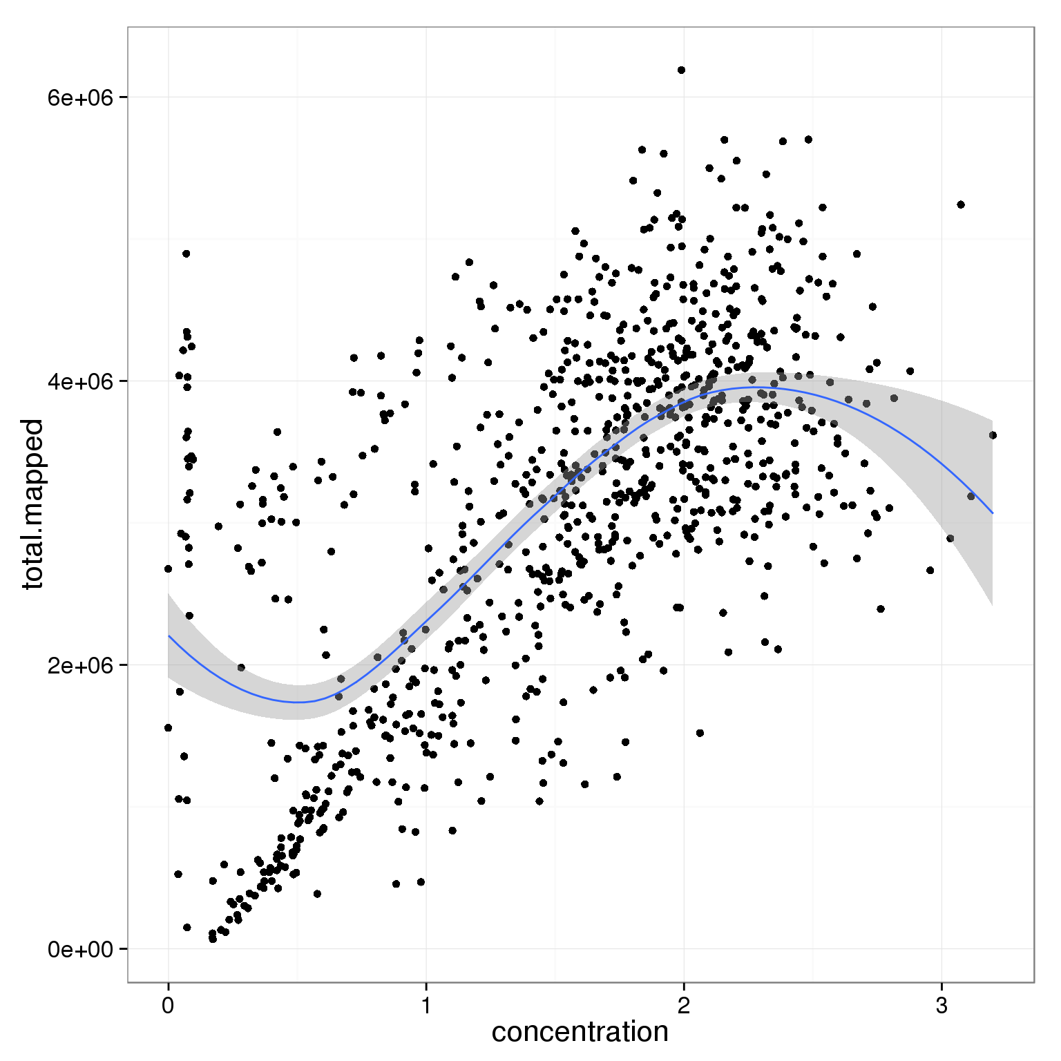
ggplot(summary_per_sample_reads_single_qc,
       aes(x = concentration, y = total_gene_molecule)) +
  geom_point() +
  geom_smooth()
geom_smooth: method="auto" and size of largest group is <1000, so using loess. Use 'method = x' to change the smoothing method.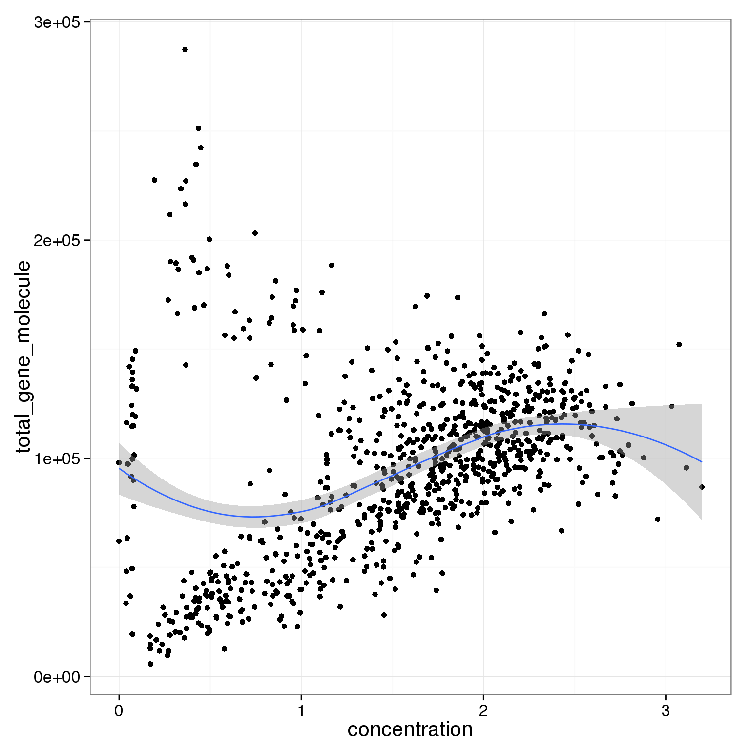
Tra-1-60
Tra-1-60 is a stem cell marker.
table(summary_per_sample_reads_single_qc$tra1.60)
  0   1
 39 825
ggplot(summary_per_sample_reads_single_qc,
aes(x = as.factor(tra1.60), y = ERCC.ratios)) +
geom_boxplot()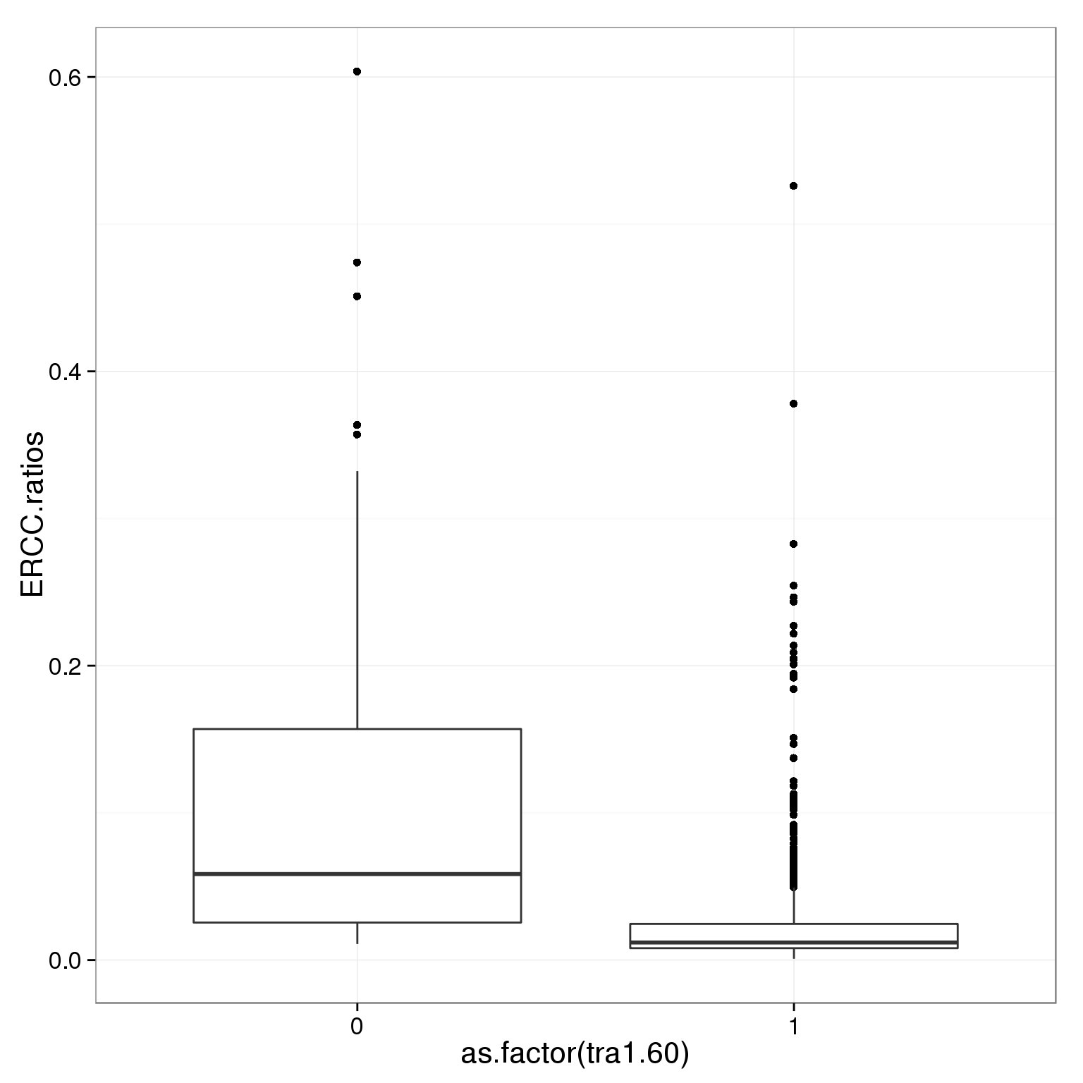
ggplot(summary_per_sample_reads_single_qc,
       aes(x = as.factor(tra1.60), y = unmapped.ratios)) +
  geom_boxplot()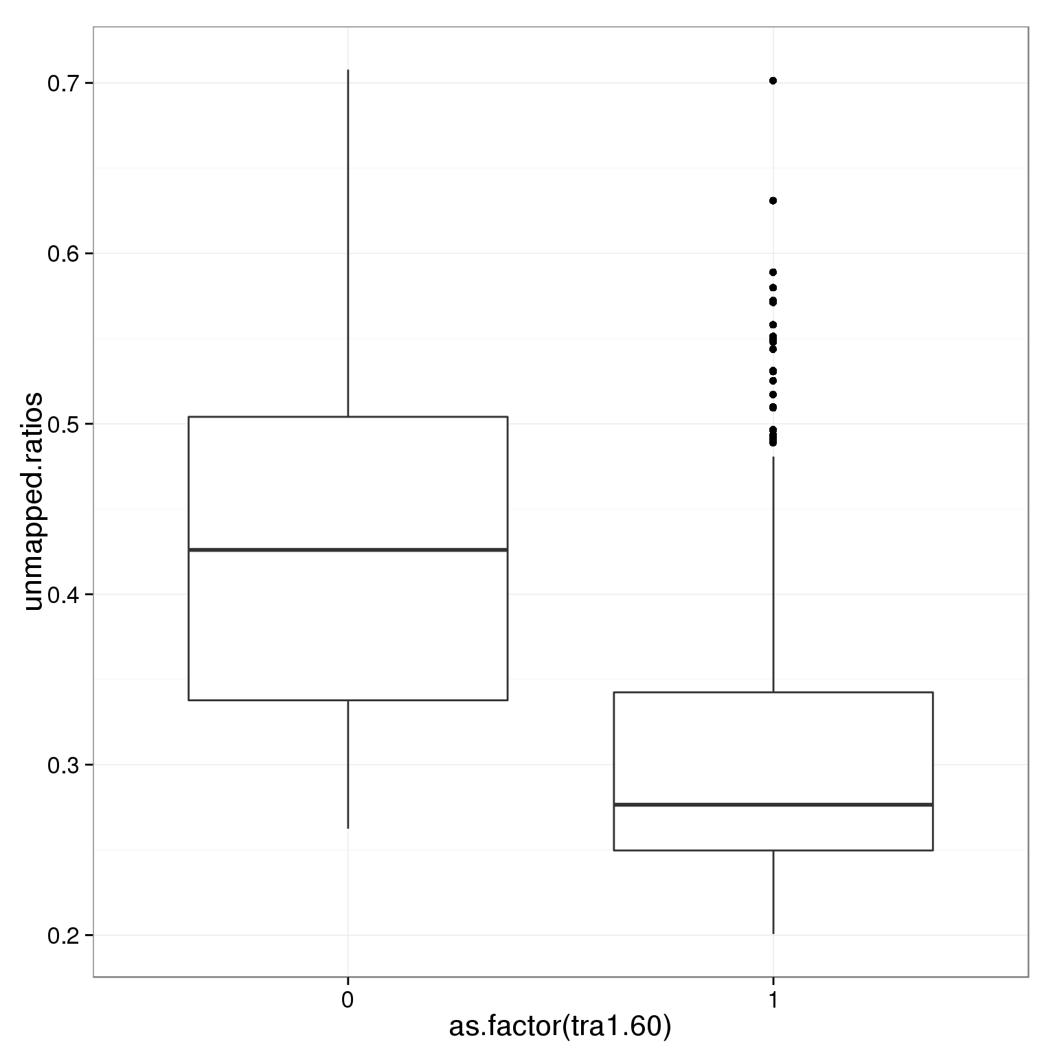
Filtering by cell number and Tra-1-60
Simply removing all the cells with bad cell number or tra-1-60 does not remove all the low quality samples.
table(summary_per_sample_reads_single_qc$cell_number,
      summary_per_sample_reads_single_qc$tra1.60)
      0   1
  0  20   1
  1  19 770
  2   0  29
  3   0  17
  4   0   3
  5   0   5
ggplot(subset(summary_per_sample_reads_single_qc, cell_number == 1 & tra1.60 == 1),
aes(x = total.mapped, y = ERCC.ratios)) +
geom_point()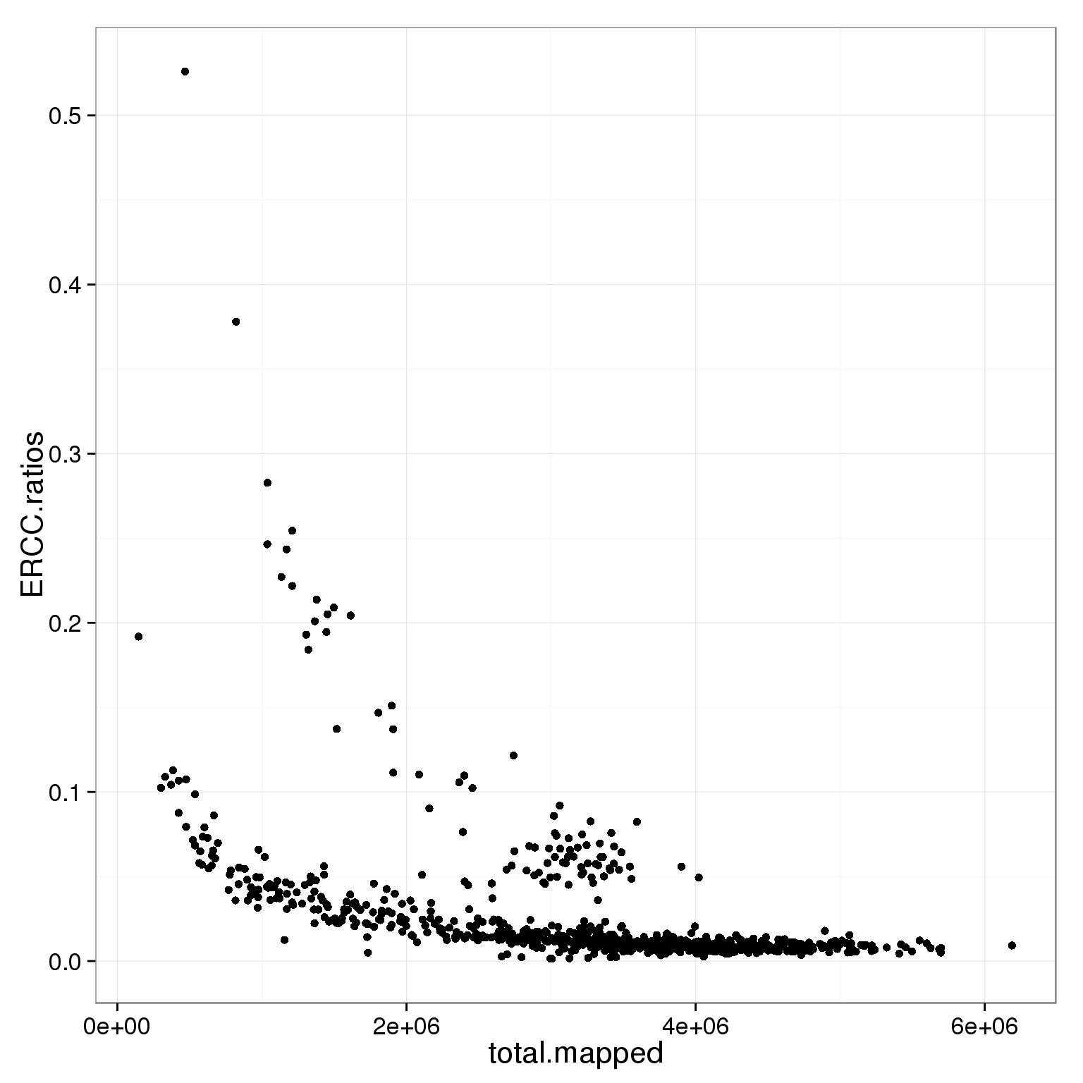
ggplot(subset(summary_per_sample_reads_single_qc, cell_number == 1 & tra1.60 == 1),
       aes(x = total.mapped, y = unmapped.ratios)) +
  geom_point()
PCA
Reads
Calculate the counts per million for the singe cells.
reads_cells_cpm <- cpm(reads)Select the most variable genes.
reads_cells_cpm_log_var <- log(apply(reads_cells_cpm, 1, var))
hist(reads_cells_cpm_log_var)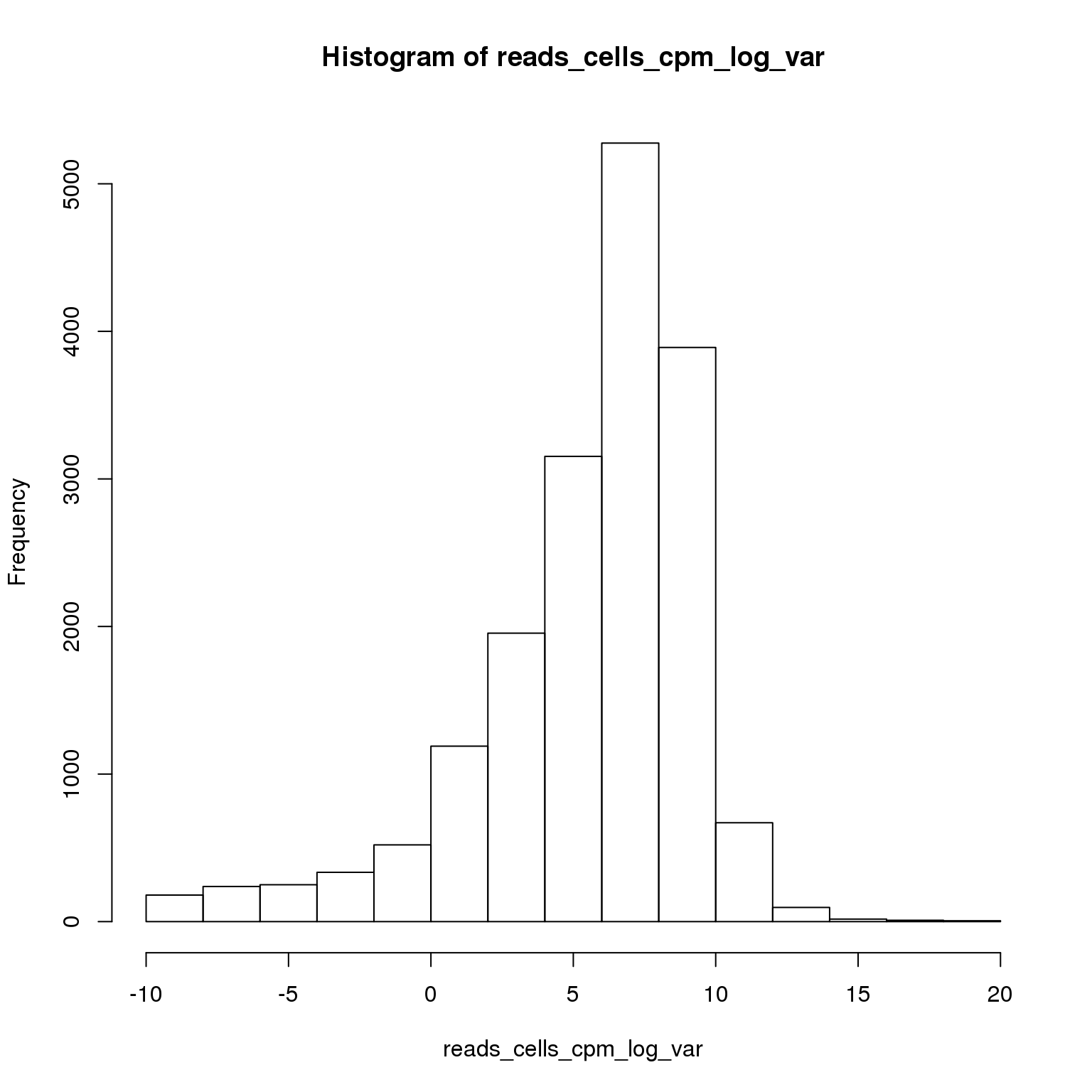
sum(reads_cells_cpm_log_var > 8)[1] 4689Using the 4689 most variable genes, perform PCA.
reads_cells_cpm <- reads_cells_cpm[reads_cells_cpm_log_var > 8, ]
pca_reads_cells <- prcomp(t(reads_cells_cpm), retx = TRUE, scale. = TRUE,
                          center = TRUE)
plot(pca_reads_cells)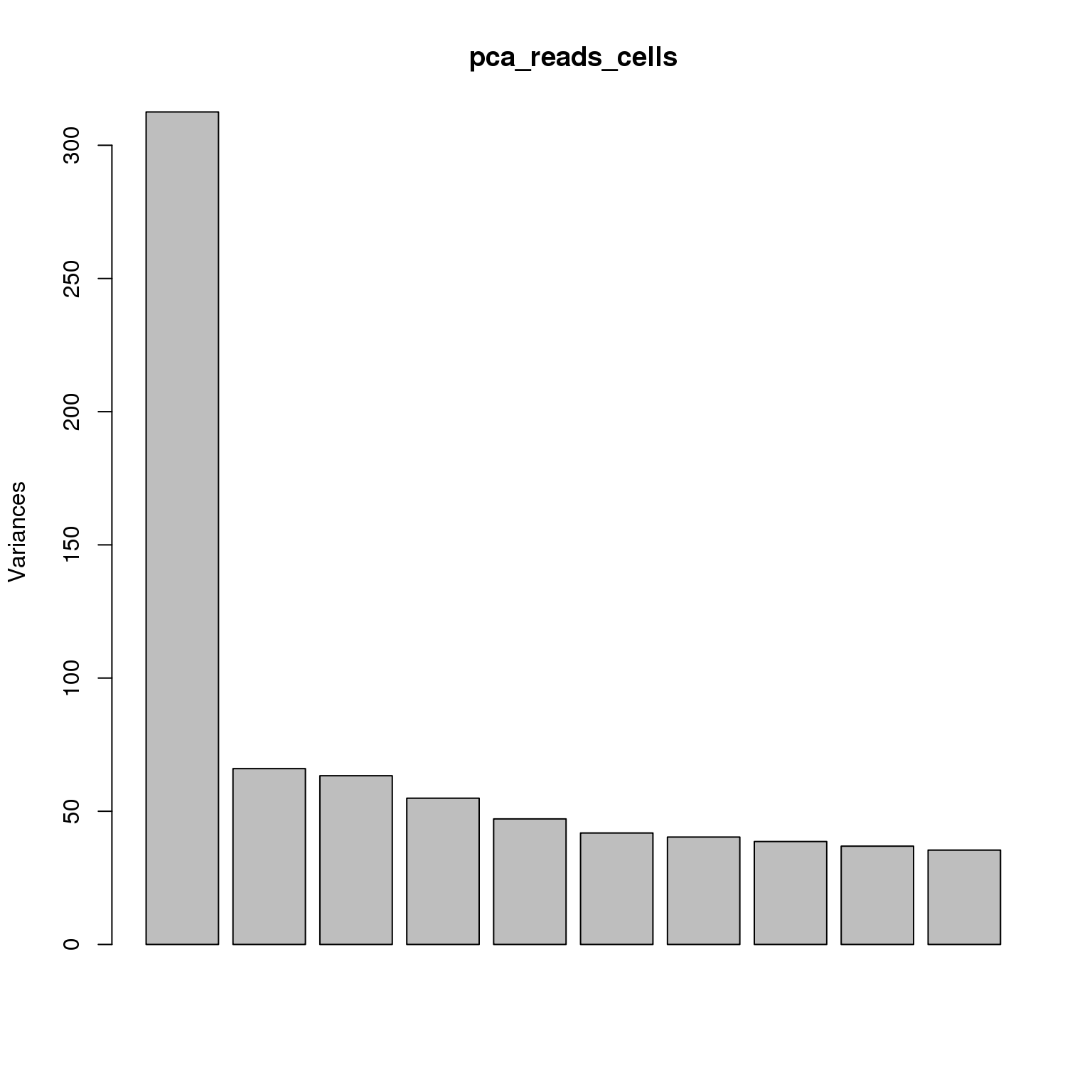
pca_reads_cells$perc_explained <- pca_reads_cells$sdev^2 / sum(pca_reads_cells$sdev^2) * 100
plot(pca_reads_cells$perc_explained)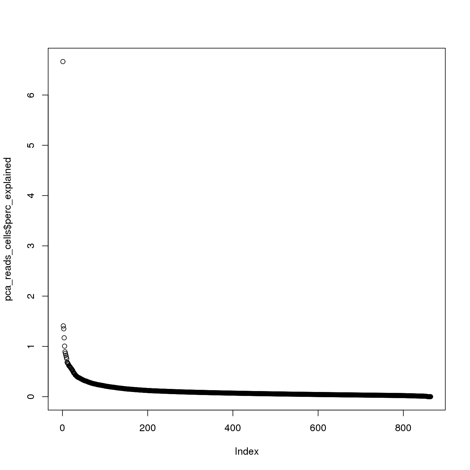
The first PC accounts for 7% of the variance and the second PC 1%.
pca_reads_cells_anno <- cbind(summary_per_sample_reads_single_qc, pca_reads_cells$x)ggplot(pca_reads_cells_anno, aes(x = PC1, y = PC2, col = as.factor(individual),
shape = as.factor(batch))) +
geom_point()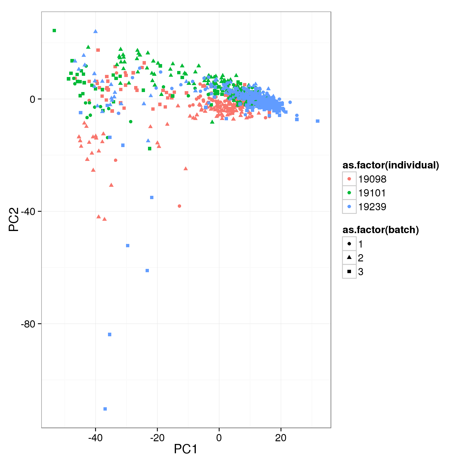
What effect is PC1 capturing?
ggplot(pca_reads_cells_anno, aes(x = as.factor(individual), y = PC1)) +
  geom_boxplot() + facet_wrap(~batch)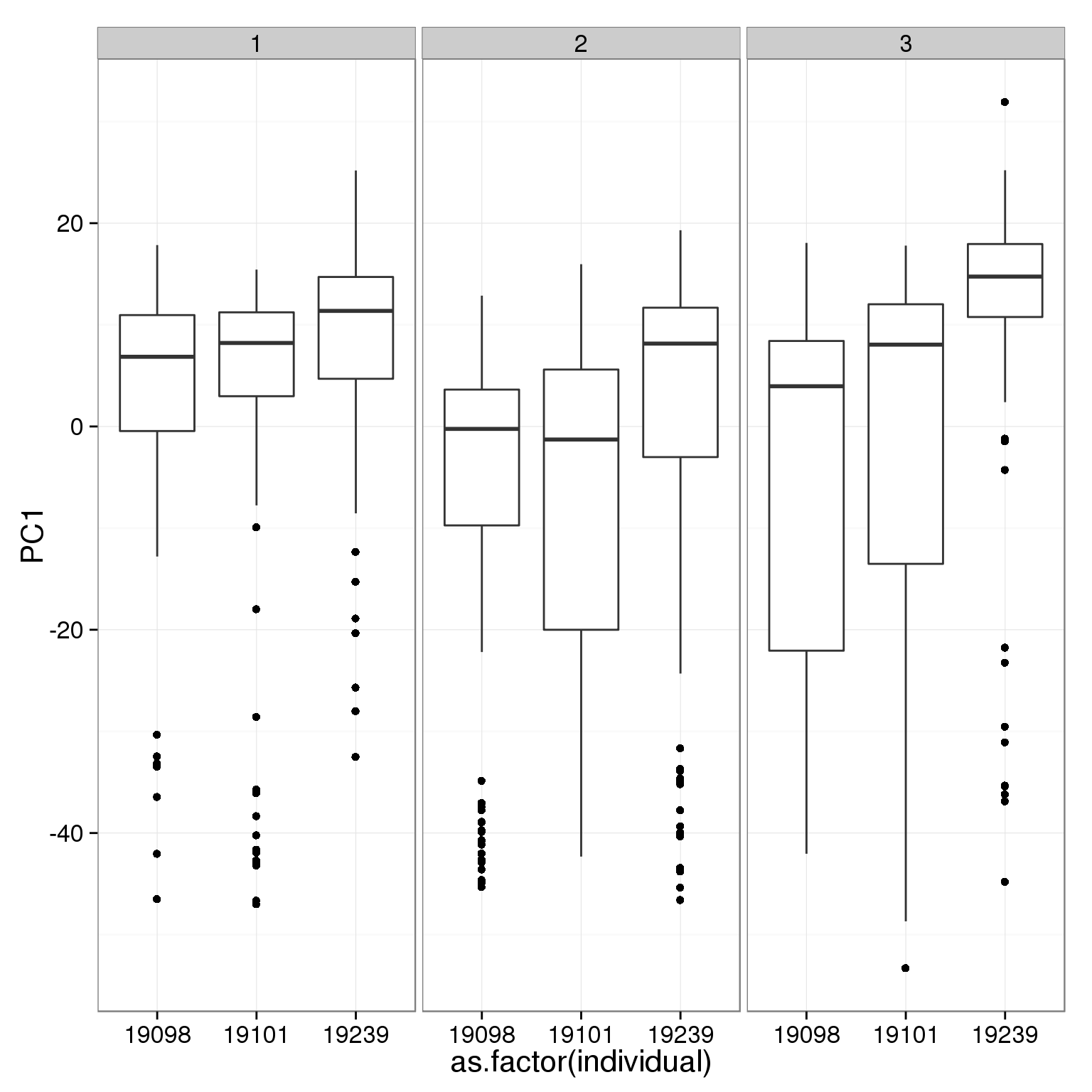
ggplot(pca_reads_cells_anno, aes(x = as.factor(batch), y = PC1)) +
  geom_boxplot() + facet_wrap(~individual)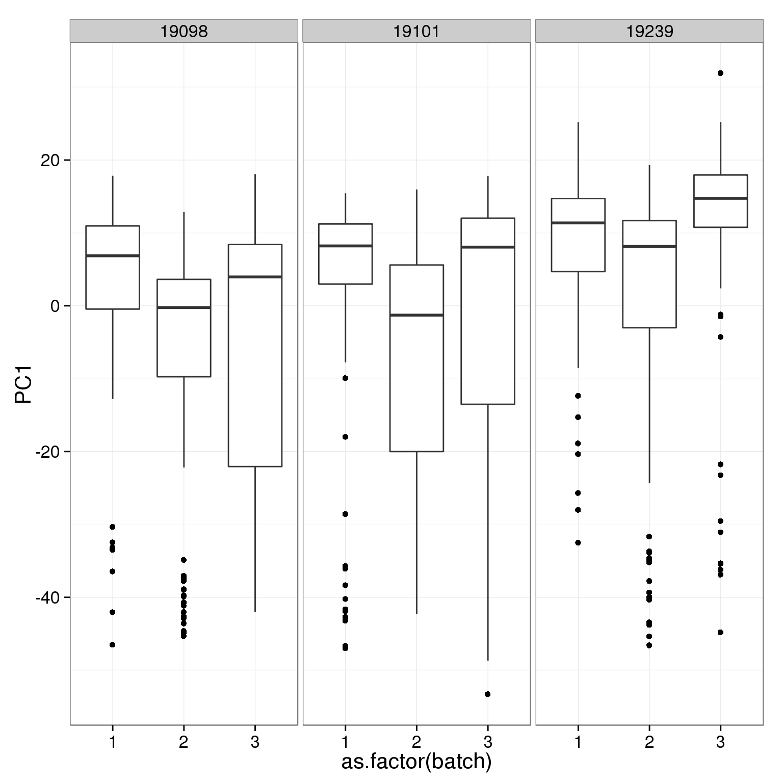
ggplot(pca_reads_cells_anno, aes(x = PC1, y = PC2)) +
  geom_text(aes(label = cell_number))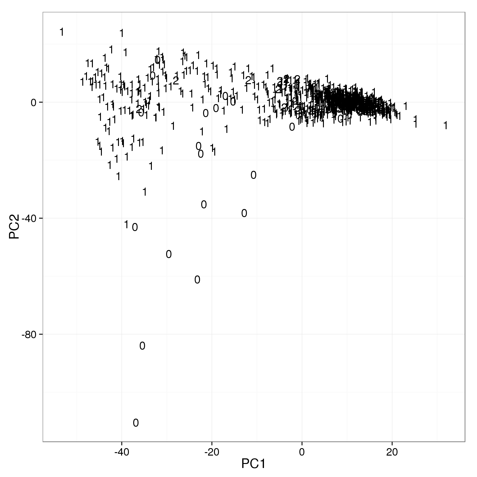
The outliers on PC2 are mainly empty wells.
ggplot(pca_reads_cells_anno, aes(x = ERCC.ratios, y = PC1)) +
  geom_point()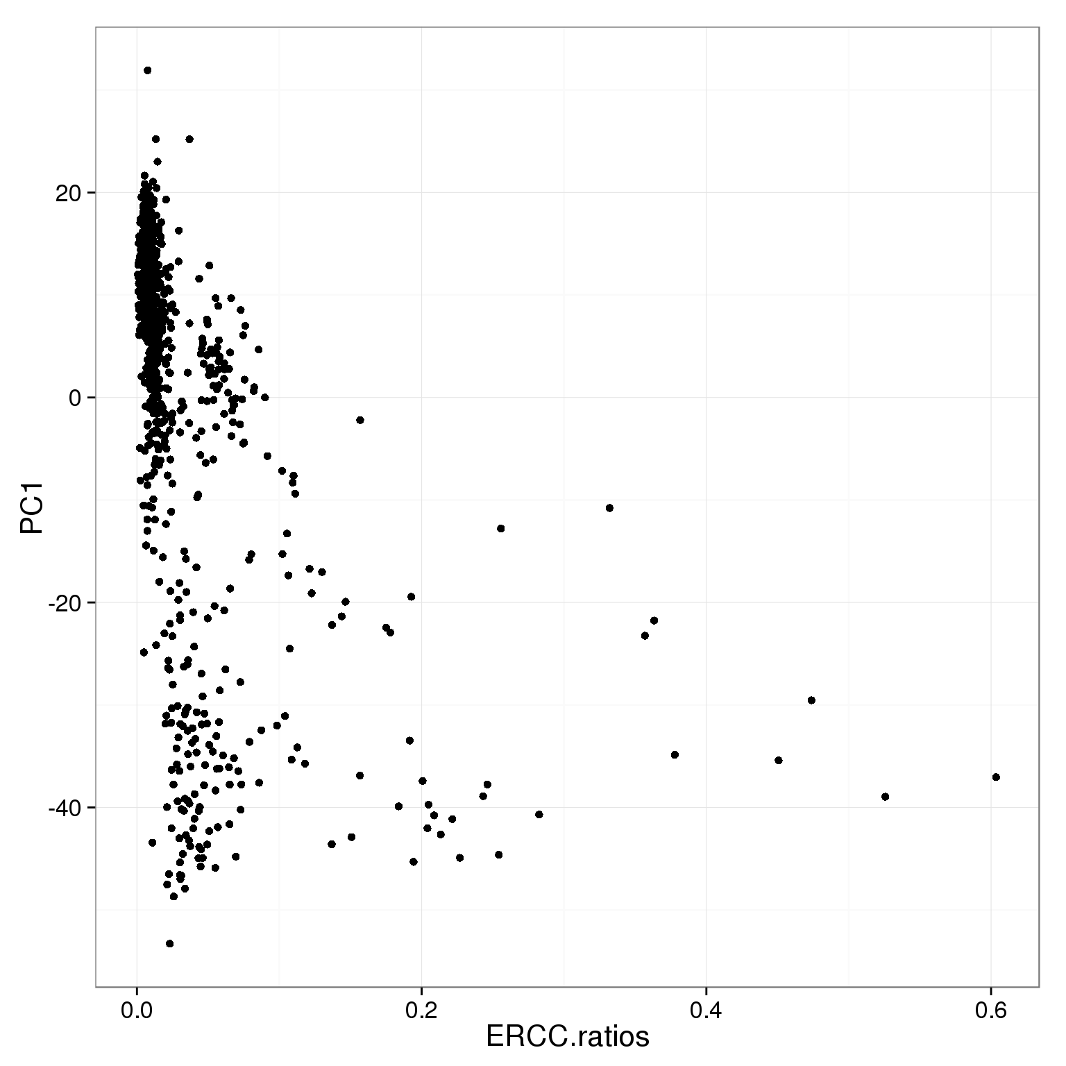
PC1 is negatively correlated with the ratio of unmapped reads.
ggplot(pca_reads_cells_anno, aes(x = unmapped.ratios, y = PC1)) +
  geom_point() +
  geom_smooth()
geom_smooth: method="auto" and size of largest group is <1000, so using loess. Use 'method = x' to change the smoothing method.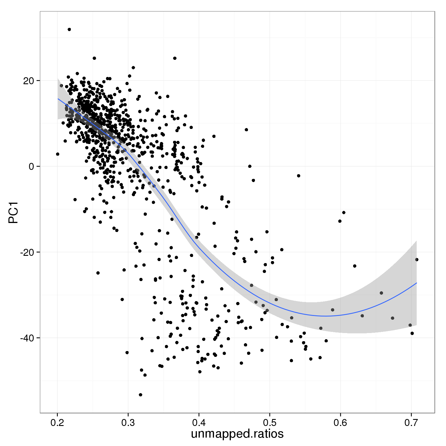
PC1 is positively correlated with the total number of mapped reads.
ggplot(pca_reads_cells_anno, aes(x = total.mapped, y = PC1)) +
  geom_point() +
  geom_smooth()
geom_smooth: method="auto" and size of largest group is <1000, so using loess. Use 'method = x' to change the smoothing method.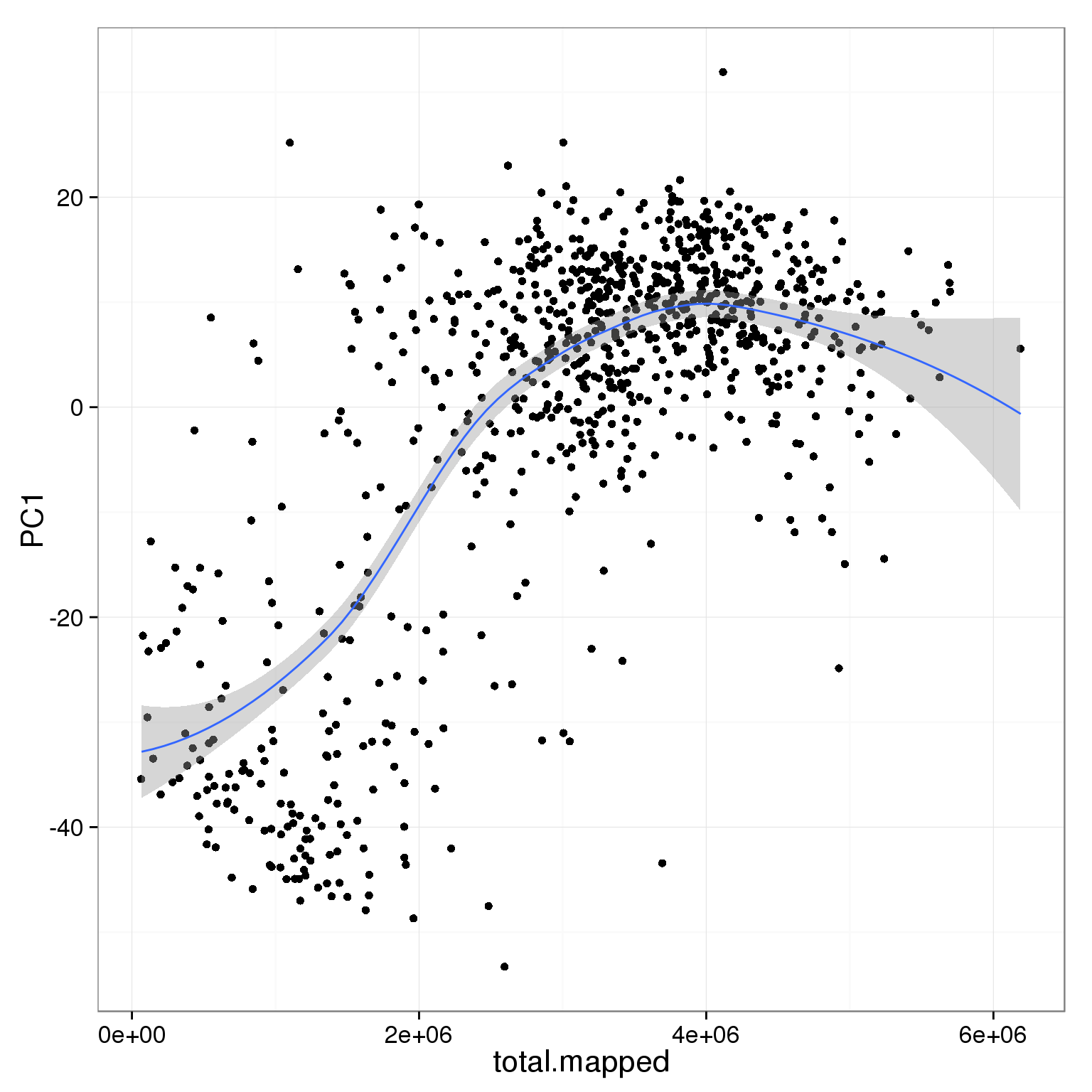
PC1 is positively correlated with the detected gene number
ggplot(pca_reads_cells_anno, aes(x = reads_single_gene_number, y = PC1)) +
  geom_point() +
  geom_smooth()
geom_smooth: method="auto" and size of largest group is <1000, so using loess. Use 'method = x' to change the smoothing method.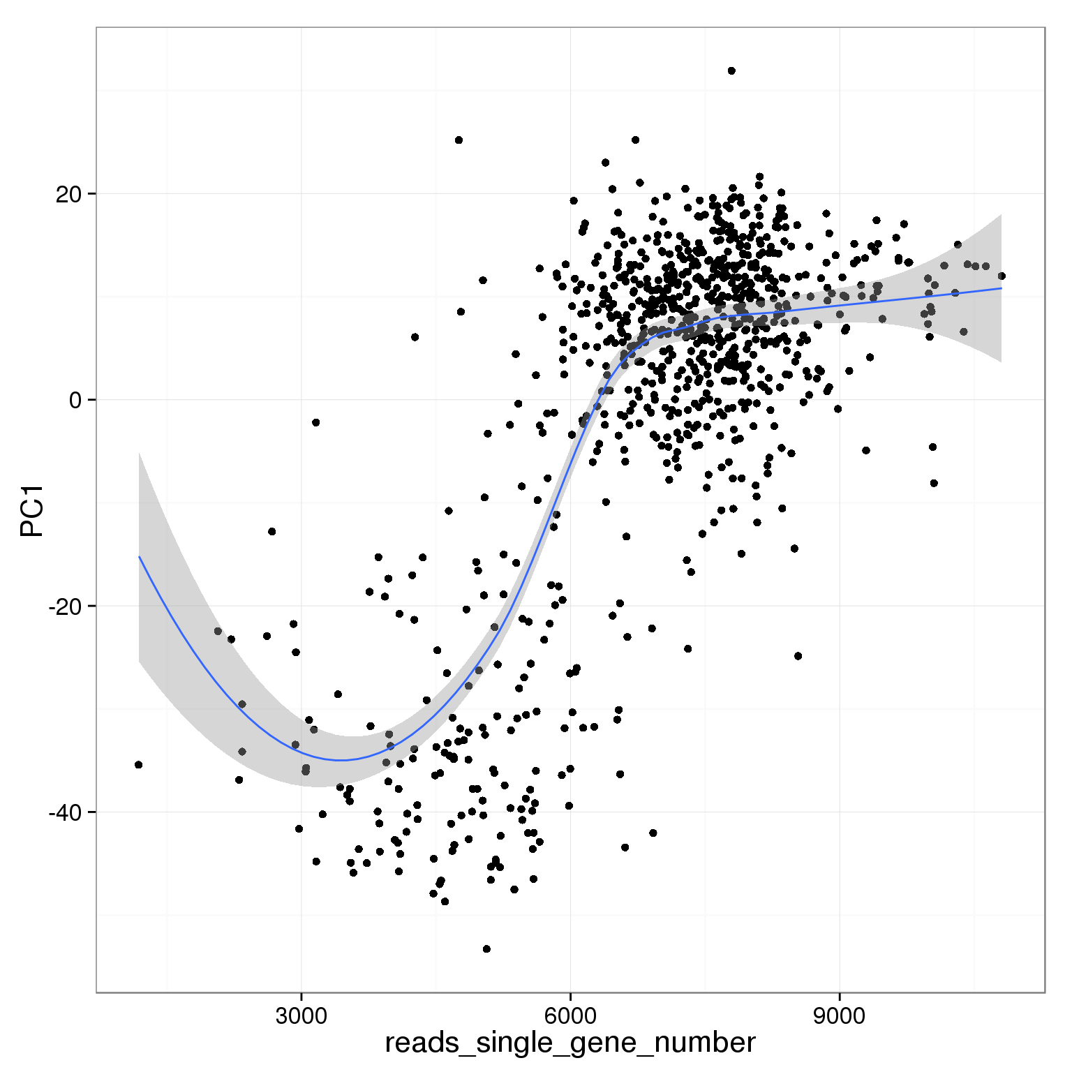
PC1 is negatively correlated with the ratio of mitochondrial reads
ggplot(pca_reads_cells_anno, aes(x = mt_reads_ratio, y = PC1)) +
  geom_point() +
  geom_smooth()
geom_smooth: method="auto" and size of largest group is <1000, so using loess. Use 'method = x' to change the smoothing method.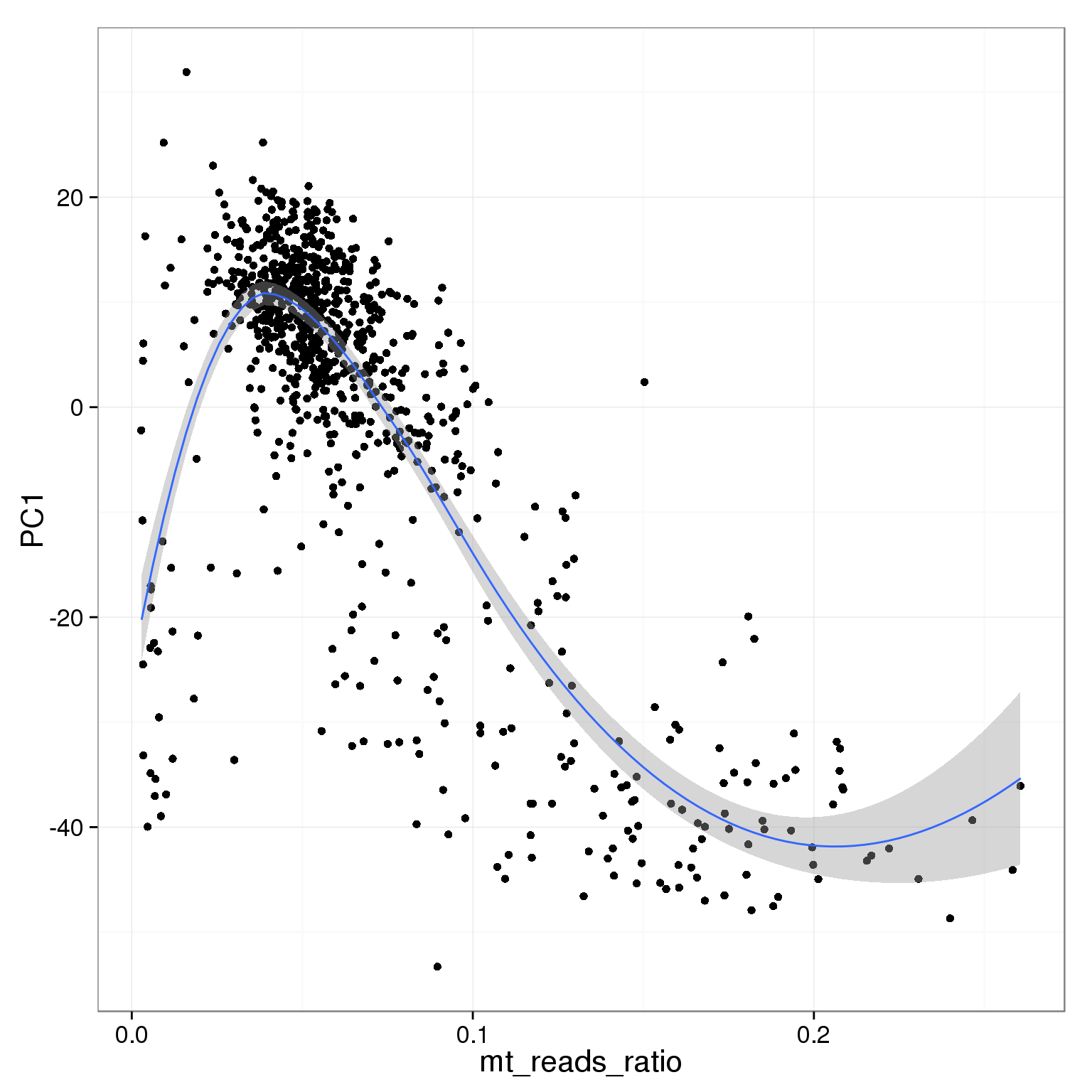
Using various simple filtering cutoffs, it is not possible to capture all the cells that have low values of PC1.
pca_reads_cells_anno$cell_filter <- pca_reads_cells_anno$cell_number == 1
ggplot(pca_reads_cells_anno, aes(x = PC1, y = PC2, col = cell_filter)) +
  geom_point()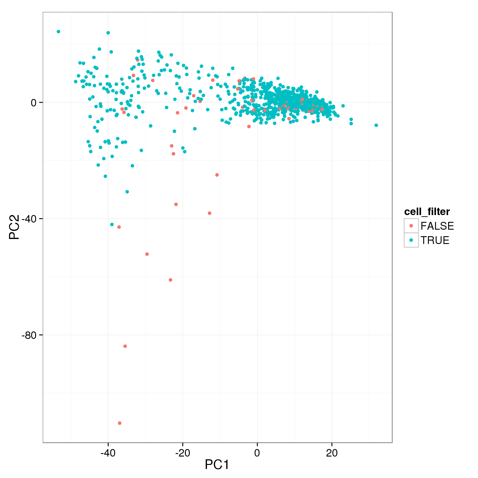
pca_reads_cells_anno$total_cutoff <- pca_reads_cells_anno$total.mapped > 1.5 * 10^6
ggplot(pca_reads_cells_anno, aes(x = PC1, y = PC2, col = total_cutoff)) +
  geom_point()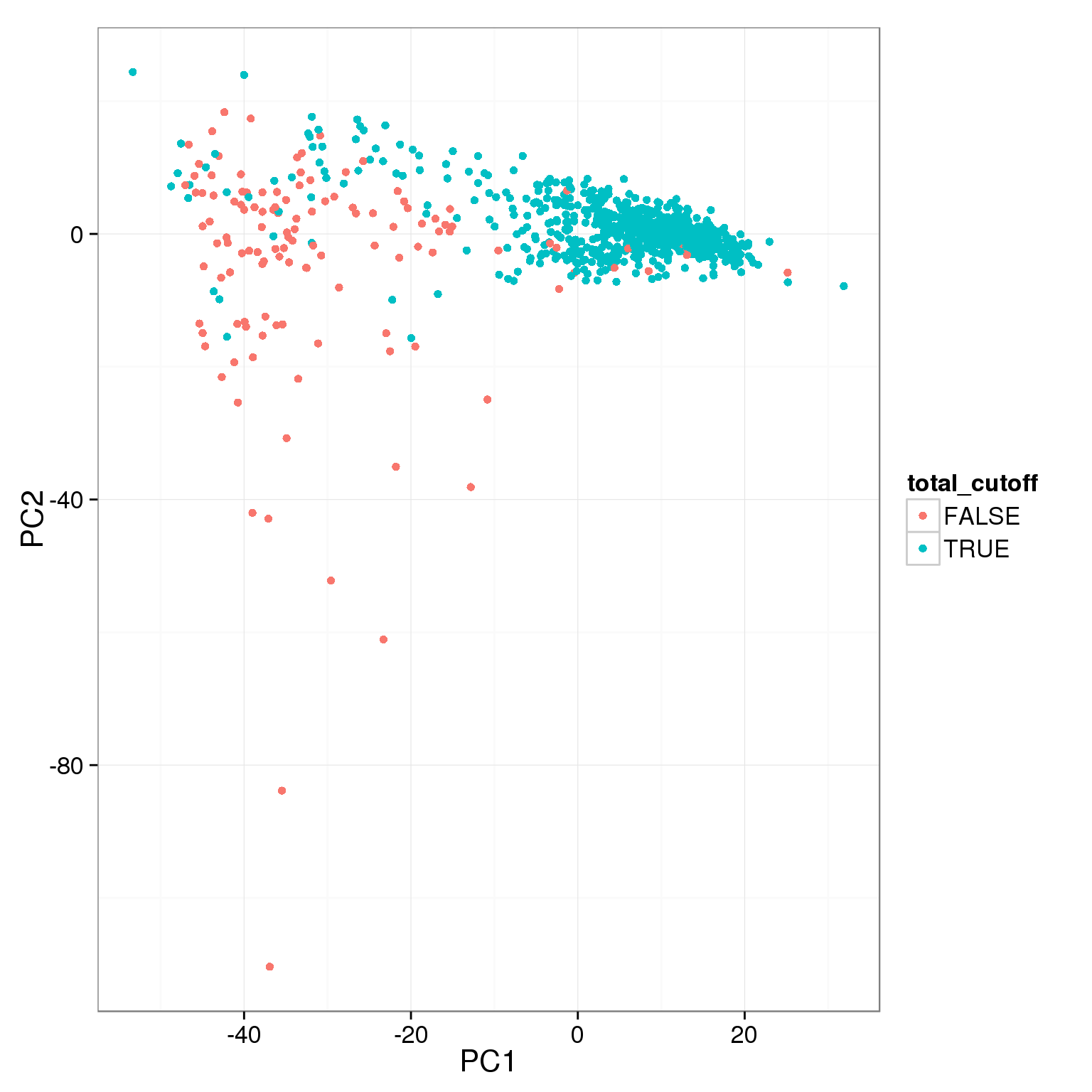
pca_reads_cells_anno$unmapped_cutoff <- pca_reads_cells_anno$unmapped.ratios < 0.4
ggplot(pca_reads_cells_anno, aes(x = PC1, y = PC2, col = unmapped_cutoff)) +
  geom_point()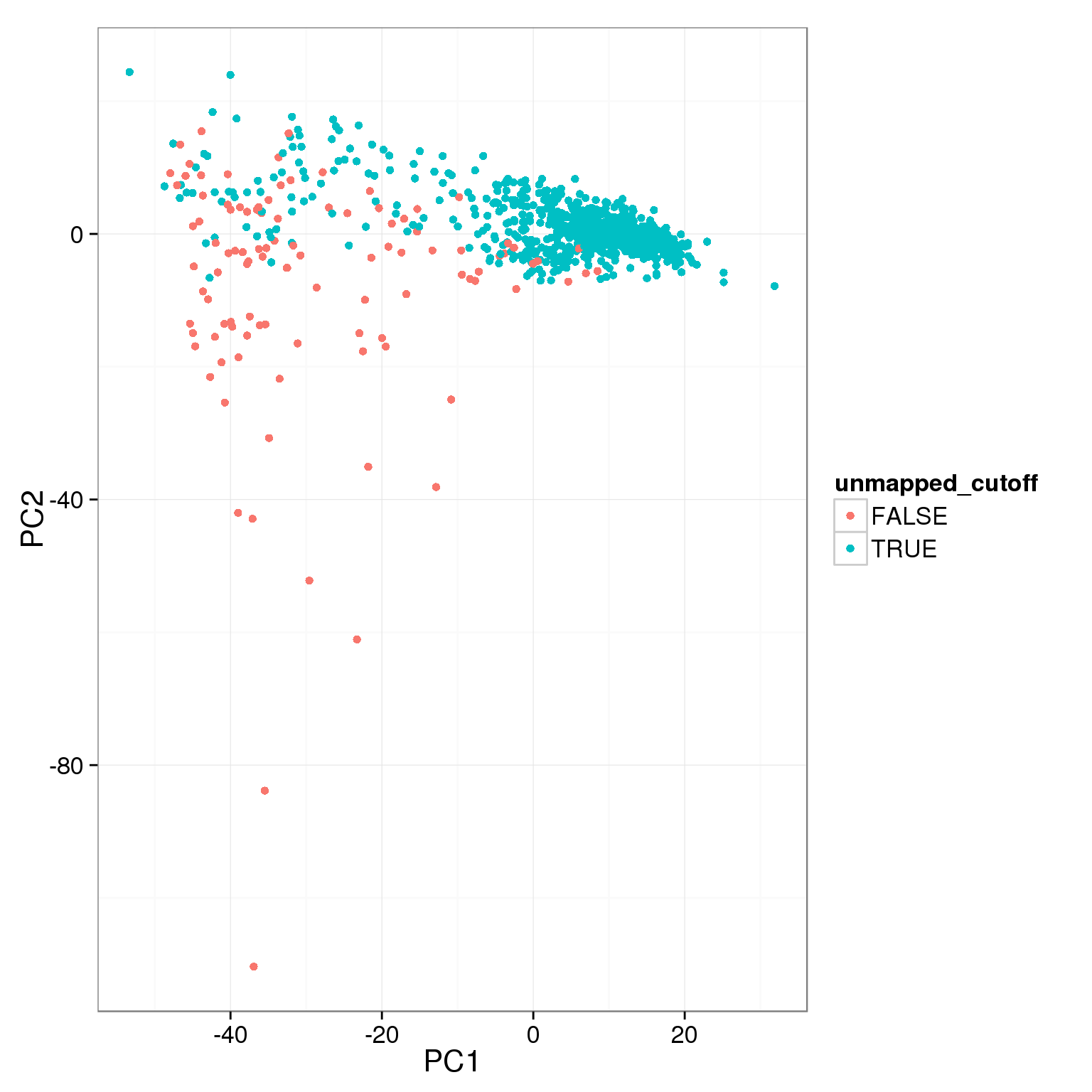
pca_reads_cells_anno$ERCC_cutoff <- pca_reads_cells_anno$ERCC.ratios < 0.05
ggplot(pca_reads_cells_anno, aes(x = PC1, y = PC2, col = ERCC_cutoff)) +
  geom_point()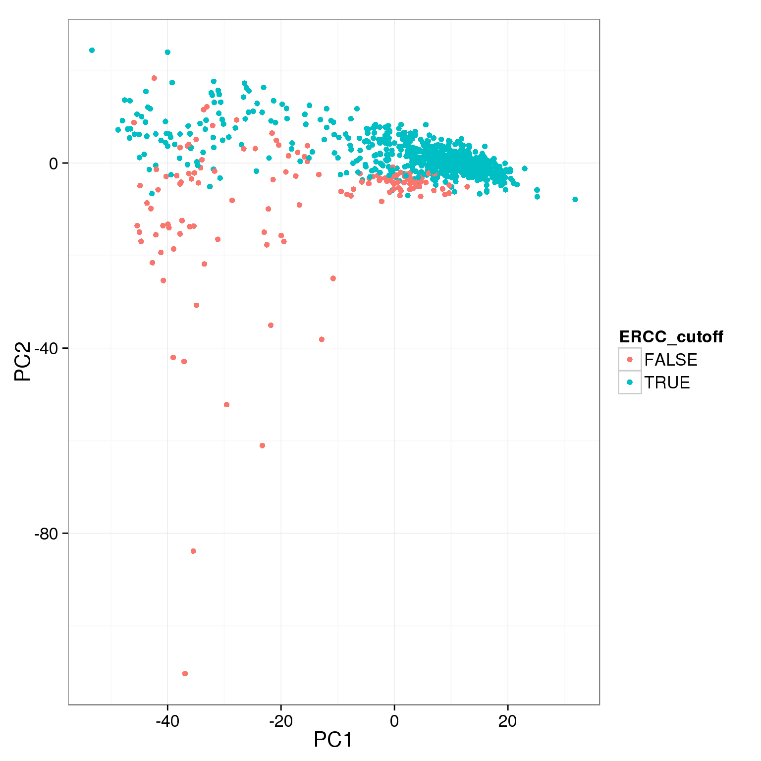
pca_reads_cells_anno$gene_filter <- pca_reads_cells_anno$reads_single_gene_number  > 6000
ggplot(pca_reads_cells_anno, aes(x = PC1, y = PC2, col = gene_filter)) +
  geom_point()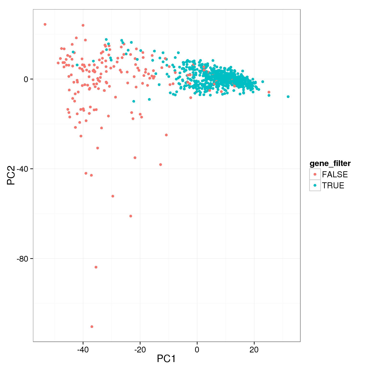
pca_reads_cells_anno$mt_filter <- pca_reads_cells_anno$mt_reads_ratio < 0.15
ggplot(pca_reads_cells_anno, aes(x = PC1, y = PC2, col = mt_filter)) +
  geom_point()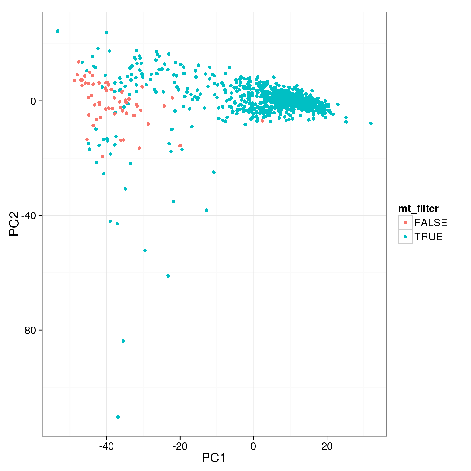
Filter
The two cutoffs, total reads and cell number, largely overlap.
table(pca_reads_cells_anno$cell_filter, pca_reads_cells_anno$total_cutoff,
      dnn = c("Num cells == 1", "Total reads > 1.5e6"))
Total reads > 1.5e6
Num cells == 1 FALSE TRUE
FALSE 20 55
TRUE 104 685Add the third cutoff, 6000 genes detected, help a bit.
pca_reads_cells_anno$qc_filter <- pca_reads_cells_anno$total_cutoff &
                                  pca_reads_cells_anno$gene_filter &
                                  pca_reads_cells_anno$cell_filter

ggplot(pca_reads_cells_anno, aes(x = PC1, y = PC2, col = qc_filter,
                                 label = as.character(cell_number))) +
  geom_text(fontface=3)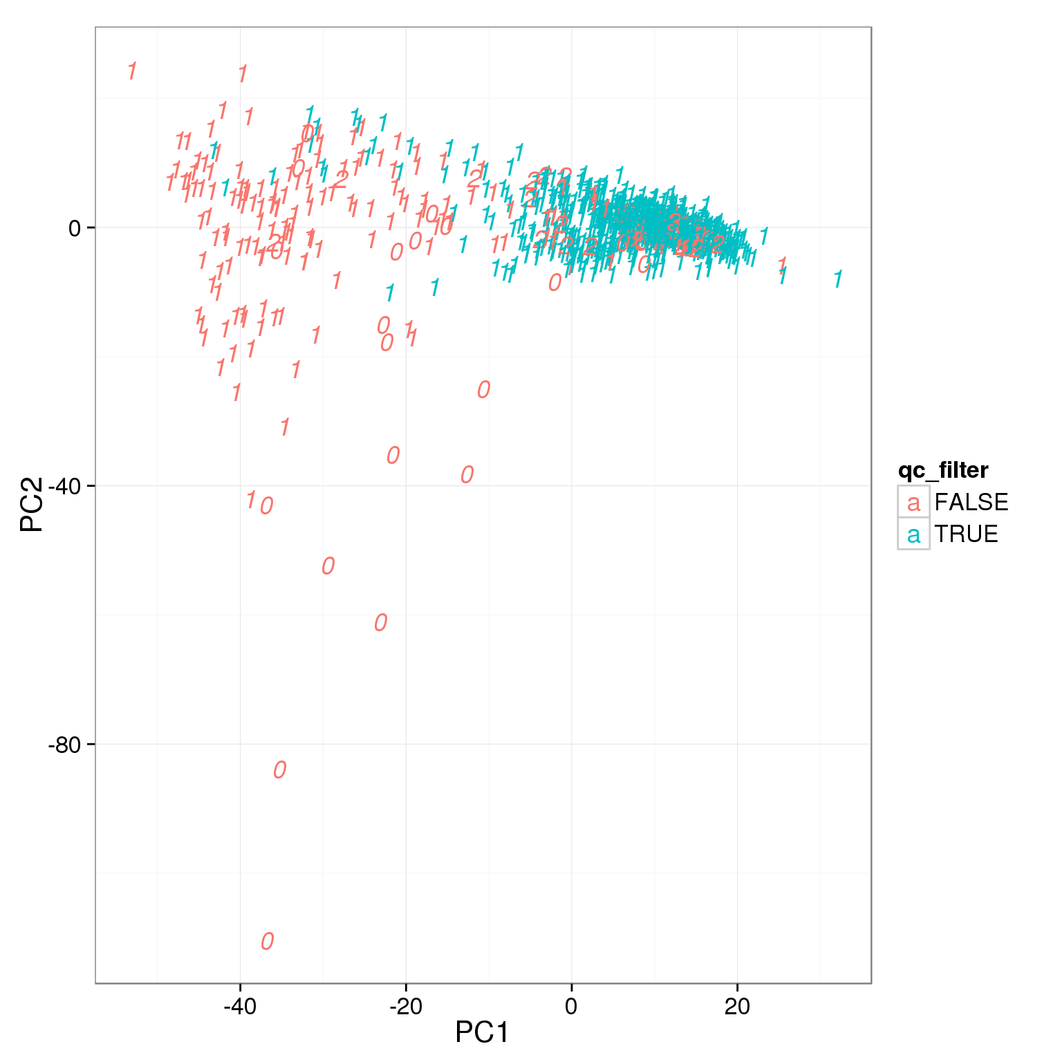
Apply all the cutoffs
pca_reads_cells_anno$qc_filter_all <- pca_reads_cells_anno$cell_filter &
                                      pca_reads_cells_anno$total_cutoff &
                                      pca_reads_cells_anno$unmapped_cutoff &
                                      pca_reads_cells_anno$ERCC_cutoff &
                                      pca_reads_cells_anno$gene_filter &
                                      pca_reads_cells_anno$mt_filter

ggplot(pca_reads_cells_anno, aes(x = PC1, y = PC2, col = qc_filter_all,
                                 label = as.character(cell_number))) +
  geom_text(fontface=3)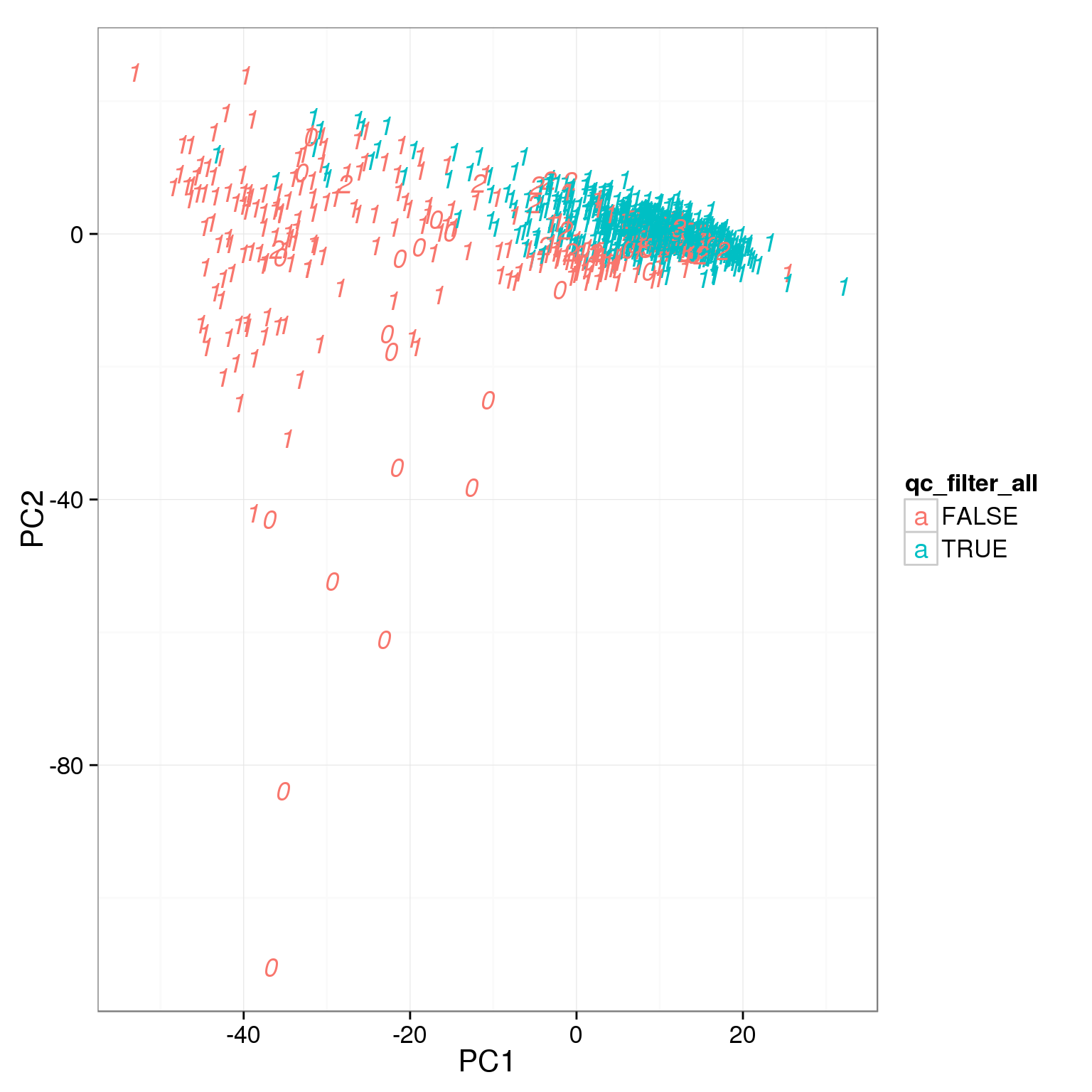
How many cells do we keep from each individual and batch using this filter?
table(pca_reads_cells_anno[pca_reads_cells_anno$qc_filter,
                           c("individual", "batch")])
batch
individual 1 2 3
19098 85 71 58
19101 77 68 52
19239 78 67 80table(pca_reads_cells_anno[pca_reads_cells_anno$qc_filter_all,
c("individual", "batch")]) batch
individual 1 2 3
19098 85 15 57
19101 77 68 52
19239 78 67 79Output list of single cells to keep.
stopifnot(nrow(pca_reads_cells_anno) == nrow(anno[anno$well != "bulk", ]))
quality_single_cells <- anno %>%
  filter(well != "bulk") %>%
  filter(pca_reads_cells_anno$qc_filter_all) %>%
  select(sample_id)
stopifnot(!grepl("bulk", quality_single_cells$sample_id))
write.table(quality_single_cells,
            file = "../data/quality-single-cells.txt", quote = FALSE,
            sep = "\t", row.names = FALSE, col.names = FALSE)
Effect of sample concentration
Investigate whether sample concentration can be reflected by total mapped reads or total molecule counts. Maybe in the bad quality cells, but not really in the good quality cells.
summary_per_sample_reads_single_qc$qc_filter_all <- pca_reads_cells_anno$qc_filter_all

ggplot(summary_per_sample_reads_single_qc,
       aes(x = concentration, y = total.mapped, col = qc_filter_all, label = as.character(cell_number))) +
  geom_text(fontface=3) +
  geom_smooth()
geom_smooth: method="auto" and size of largest group is <1000, so using loess. Use 'method = x' to change the smoothing method.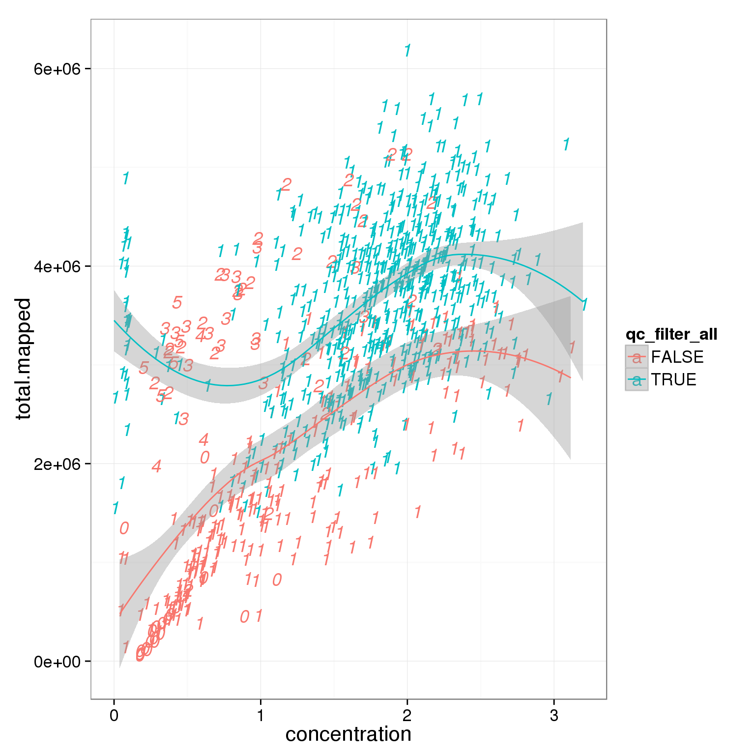
ggplot(summary_per_sample_reads_single_qc,
       aes(x = concentration, y = total_gene_molecule, col = qc_filter_all, label = as.character(cell_number))) +
  geom_text(fontface=3) +
  geom_smooth()
geom_smooth: method="auto" and size of largest group is <1000, so using loess. Use 'method = x' to change the smoothing method.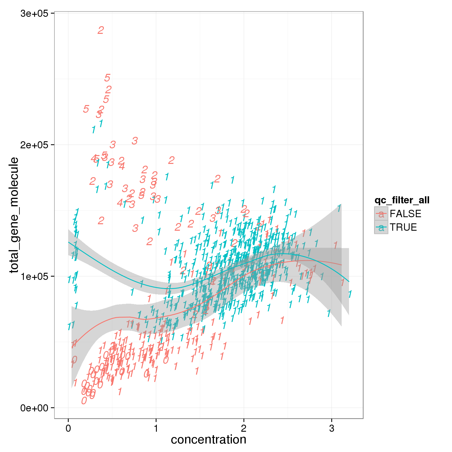
Session information
sessionInfo()R version 3.2.0 (2015-04-16)
Platform: x86_64-unknown-linux-gnu (64-bit)
locale:
[1] LC_CTYPE=en_US.UTF-8 LC_NUMERIC=C
[3] LC_TIME=en_US.UTF-8 LC_COLLATE=en_US.UTF-8
[5] LC_MONETARY=en_US.UTF-8 LC_MESSAGES=en_US.UTF-8
[7] LC_PAPER=en_US.UTF-8 LC_NAME=C
[9] LC_ADDRESS=C LC_TELEPHONE=C
[11] LC_MEASUREMENT=en_US.UTF-8 LC_IDENTIFICATION=C
attached base packages:
[1] stats graphics grDevices utils datasets methods base
other attached packages:
[1] edgeR_3.10.2 limma_3.24.9 ggplot2_1.0.1 dplyr_0.4.2 knitr_1.10.5
loaded via a namespace (and not attached):
[1] Rcpp_0.12.0 magrittr_1.5 MASS_7.3-40 munsell_0.4.2
[5] colorspace_1.2-6 R6_2.1.1 stringr_1.0.0 httr_0.6.1
[9] plyr_1.8.3 tools_3.2.0 parallel_3.2.0 grid_3.2.0
[13] gtable_0.1.2 DBI_0.3.1 htmltools_0.2.6 lazyeval_0.1.10
[17] yaml_2.1.13 assertthat_0.1 digest_0.6.8 reshape2_1.4.1
[21] formatR_1.2 bitops_1.0-6 RCurl_1.95-4.6 evaluate_0.7
[25] rmarkdown_0.6.1 labeling_0.3 stringi_0.4-1 scales_0.2.4
[29] proto_0.3-10