Quality control for LCLs
2015-07-10
Last updated: 2015-08-18
Code version: 60a212f941df6f91b772339aebd682435732d8f4
This is the quality control at single cell level of 19239 LCLs. 96 cells were collected on a C1 prep. I only purchased enough Tn5 from Epicentre for the generation of transposomes with 24 different barcodes. As a results, the 96 cells were divided into four groups, each have 24 cells, for library preps (4 batches) and for sequencing (4 lanes). Additionally, 4 individual cells collected from a different C1 prep were sujected to library preps using either the Epicentre Tn5 (A9E1 and B2E2) or the home-made Tn5 (B4H1 and D2H2).
Input
library("dplyr")
library("ggplot2")
theme_set(theme_bw(base_size = 16))
library("edgeR")
counts <- read.table("/mnt/gluster/data/internal_supp/singleCellSeq/lcl/gene-counts-lcl.txt",
header = TRUE, sep = "\t", stringsAsFactors = FALSE)anno <- counts %>%
filter(rmdup == "molecules") %>%
select(individual:well) %>%
arrange(well)
anno <- mutate(anno, sample_id = paste(paste0("NA", individual),
batch, well, sep = "."))
anno <- mutate(anno, full_lane = well %in% c("A9E1", "B2E2", "B4H1", "D2H2"))
stopifnot(sum(anno$full_lane) == 4)
write.table(anno, "../data/annotation-lcl.txt", quote = FALSE, sep = "\t",
row.names = FALSE)
head(anno) individual batch well sample_id full_lane
1 19239 1 A01 NA19239.1.A01 FALSE
2 19239 1 A02 NA19239.1.A02 FALSE
3 19239 1 A03 NA19239.1.A03 FALSE
4 19239 1 A04 NA19239.1.A04 FALSE
5 19239 1 A05 NA19239.1.A05 FALSE
6 19239 1 A06 NA19239.1.A06 FALSEmolecules <- counts %>%
arrange(well) %>%
filter(rmdup == "molecules") %>%
select(-(individual:rmdup)) %>%
t
dim(molecules)[1] 20419 100colnames(molecules) <- anno$sample_id
# Fix ERCC names. A data table can have dashes in column names, but data frame
# converts to period. Since the iPSC data was read with fread from the
# data.table package in sum-counts-per-sample.Rmd, this was not a problem
# before.
rownames(molecules) <- sub("\\.", "-", rownames(molecules))
write.table(molecules, "../data/molecules-lcl.txt", quote = FALSE, sep = "\t",
col.names = NA)
molecules[1:10, 1:5] NA19239.1.A01 NA19239.1.A02 NA19239.1.A03 NA19239.1.A04
ENSG00000186092 0 0 0 0
ENSG00000237683 0 0 0 0
ENSG00000235249 0 0 0 0
ENSG00000185097 0 0 0 0
ENSG00000269831 0 0 0 0
ENSG00000269308 0 0 0 0
ENSG00000187634 0 0 0 0
ENSG00000268179 0 0 0 0
ENSG00000188976 0 0 0 0
ENSG00000187961 0 0 0 0
NA19239.1.A05
ENSG00000186092 0
ENSG00000237683 0
ENSG00000235249 0
ENSG00000185097 0
ENSG00000269831 0
ENSG00000269308 0
ENSG00000187634 0
ENSG00000268179 0
ENSG00000188976 0
ENSG00000187961 0reads <- counts %>%
arrange(well) %>%
filter(rmdup == "reads") %>%
select(-(individual:rmdup)) %>%
t
dim(reads)[1] 20419 100colnames(reads) <- anno$sample_id
rownames(reads) <- sub("\\.", "-", rownames(reads))
write.table(reads, "../data/reads-lcl.txt", quote = FALSE, sep = "\t",
col.names = NA)
reads[1:10, 1:5] NA19239.1.A01 NA19239.1.A02 NA19239.1.A03 NA19239.1.A04
ENSG00000186092 0 0 0 0
ENSG00000237683 0 0 0 0
ENSG00000235249 0 0 0 0
ENSG00000185097 0 0 0 0
ENSG00000269831 0 0 0 0
ENSG00000269308 0 0 0 0
ENSG00000187634 0 0 0 0
ENSG00000268179 0 0 0 0
ENSG00000188976 0 0 0 0
ENSG00000187961 0 0 0 0
NA19239.1.A05
ENSG00000186092 0
ENSG00000237683 0
ENSG00000235249 0
ENSG00000185097 0
ENSG00000269831 0
ENSG00000269308 0
ENSG00000187634 0
ENSG00000268179 0
ENSG00000188976 0
ENSG00000187961 0Summary counts from featureCounts. Created with gather-summary-counts.py. These data were collected from the summary files of the full combined samples.
summary_counts <- read.table("../data/summary-counts-lcl.txt", header = TRUE,
                             stringsAsFactors = FALSE)
Currently this file only contains data from sickle-trimmed reads, so the code below simply ensures this and then removes the column.
summary_per_sample <- summary_counts %>%
  filter(sickle == "quality-trimmed") %>%
  select(-sickle) %>%
  arrange(individual, batch, well, rmdup)
stopifnot(summary_per_sample$well[c(TRUE, FALSE)] == anno$well)
Input single cell observational quality control data.
# File needs to be created
qc <- read.csv("../data/qc-lcl.csv", header = TRUE,
                 stringsAsFactors = FALSE)
head(qc)
X ll_name cell.number.location cell.num
1 1 A01 1_C03 1
2 2 A02 1_C02 1
3 3 A03 0_C01 0
4 4 A04 1_C49 1
5 5 A05 1_C50 1
6 6 A06 1_C51 1Total mapped reads, unmapped ratios, and ERCC ratios
Looking at the unmapped ratio and ERCC ratio of each cell based on number of reads.
# reads per sample
summary_per_sample_reads <- summary_per_sample %>% filter(rmdup == "reads")

# create unmapped ratios
summary_per_sample_reads$unmapped.ratios <- summary_per_sample_reads[,9]/apply(summary_per_sample_reads[,5:13],1,sum)

# create total mapped reads
summary_per_sample_reads$total.mapped <- apply(summary_per_sample_reads[,5:8],1,sum)

# plot
ggplot(summary_per_sample_reads, aes(x = total.mapped, y = unmapped.ratios, col = as.factor(individual), shape = as.factor(batch), label = well)) + geom_point(size = 3, alpha = 0.5) + geom_text()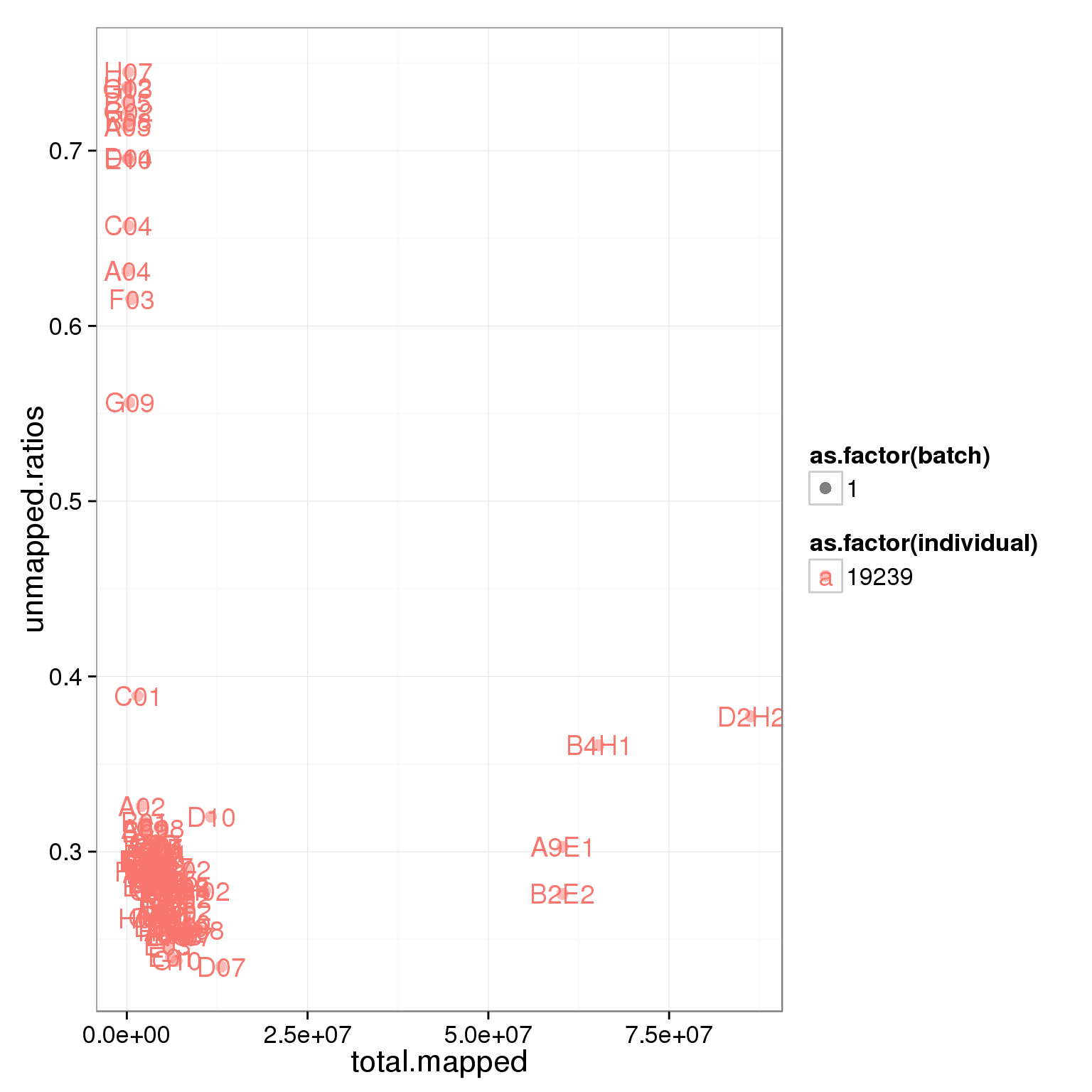
# plot the sum of reads and 'Assigned'
plot(apply(reads,2,sum),summary_per_sample_reads[,5])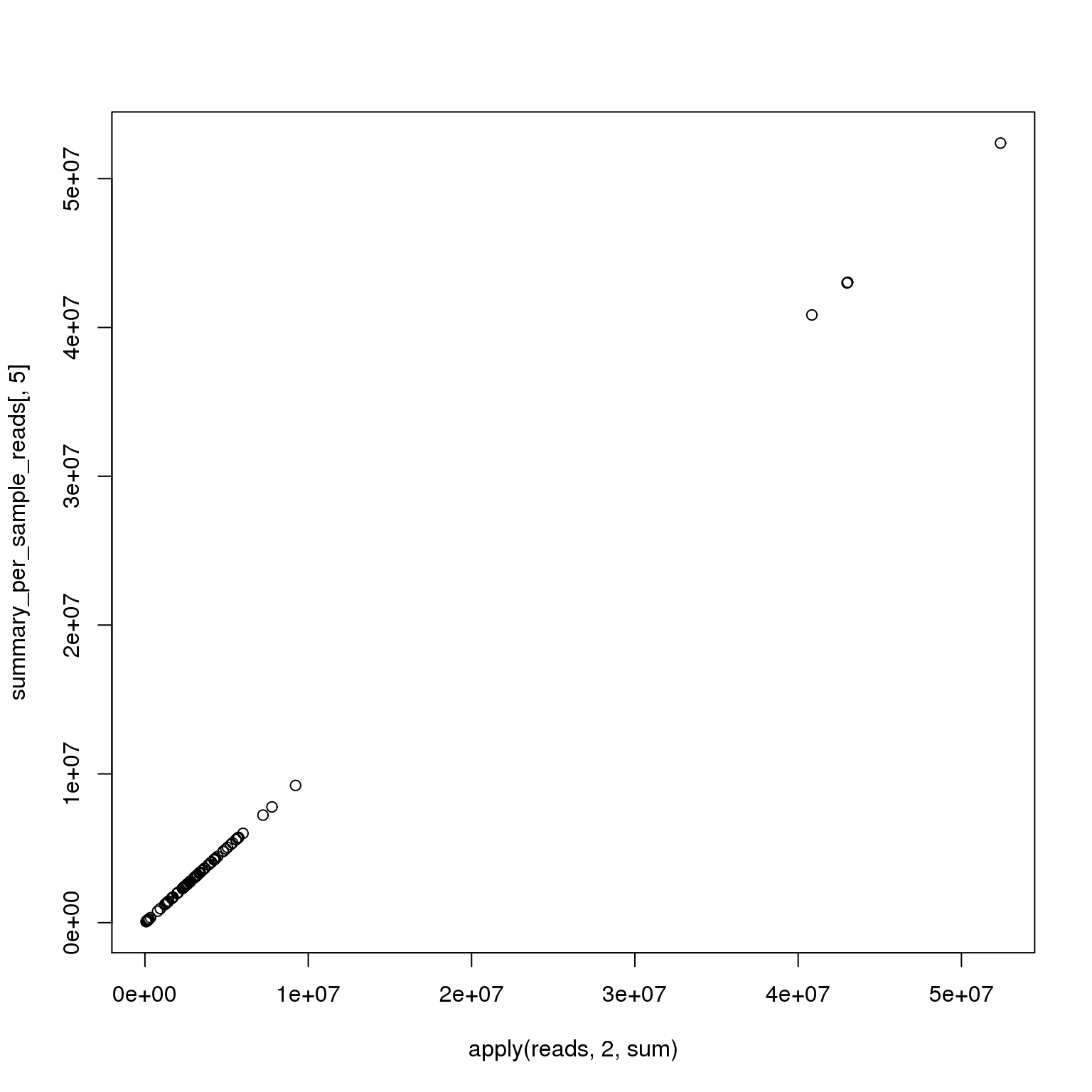
# total ERCC reads
summary_per_sample_reads$total.ERCC <- apply(reads[grep("ERCC", rownames(reads)), ],2,sum)

plot(summary_per_sample_reads$total.ERCC)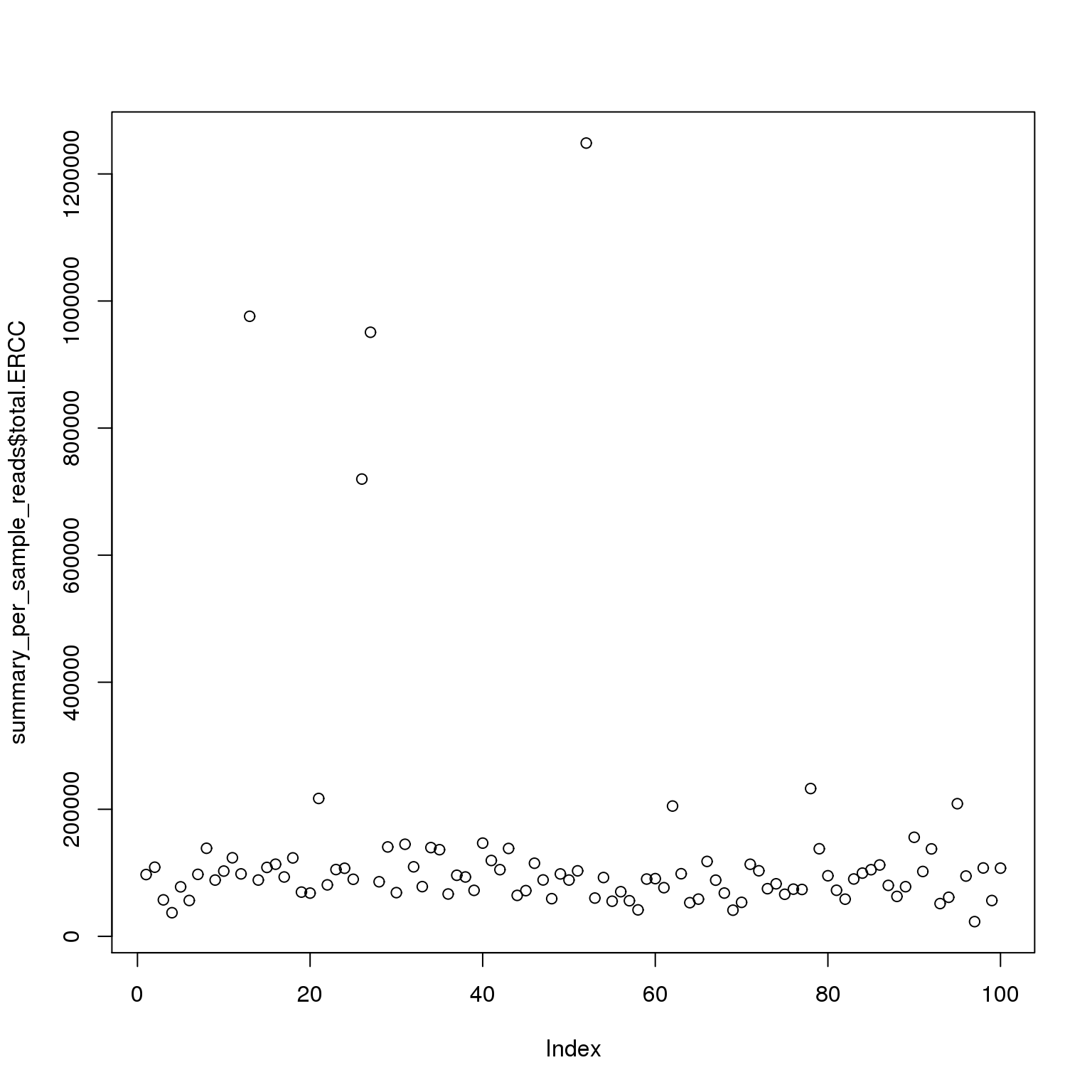
# creat ERCC ratios
summary_per_sample_reads$ERCC.ratios <- apply(reads[grep("ERCC", rownames(reads)), ],2,sum)/apply(summary_per_sample_reads[,5:8],1,sum)

# plot
ggplot(summary_per_sample_reads, aes(x = total.mapped, y = ERCC.ratios, col = as.factor(individual), shape = as.factor(batch), label = well)) + geom_point(size = 3, alpha = 0.5) + geom_text(angle = 45)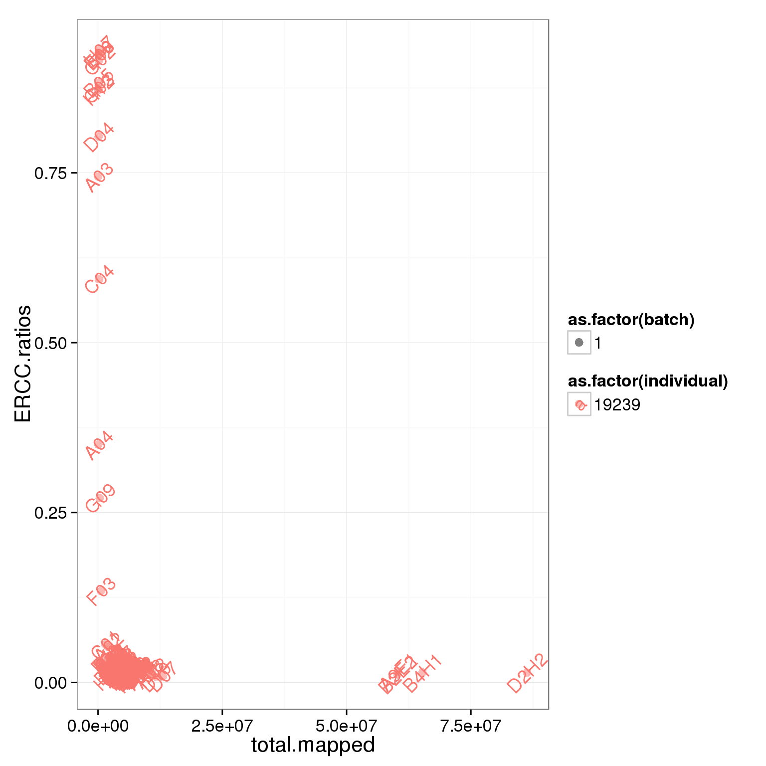
The total molecule number of ERCC and endogenous genes
summary_per_sample_reads$total_ERCC_molecule <- apply(molecules[grep("ERCC", rownames(molecules)), ],2,sum)

summary_per_sample_reads$total_gene_molecule <- apply(molecules[grep("ENSG", rownames(molecules)), ],2,sum)

ggplot(summary_per_sample_reads, aes(x = total.mapped, y = total_gene_molecule, col = as.factor(individual), shape = as.factor(batch), label = well)) + geom_point(size = 3, alpha = 0.5) + xlab("Total mapped reads") + ylab("Total gene molecule") + geom_smooth()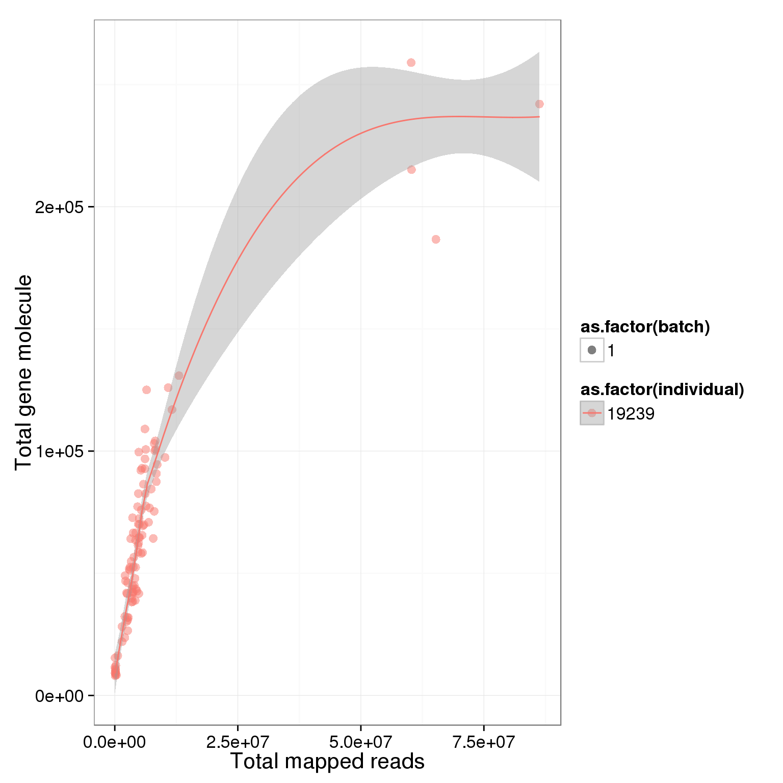
ggplot(summary_per_sample_reads, aes(x = total.mapped, y = total_ERCC_molecule, col = as.factor(individual), shape = as.factor(batch), label = well)) + geom_point(size = 3, alpha = 0.5) + xlab("Total mapped reads") + ylab("Total ERCC molecule") + geom_smooth()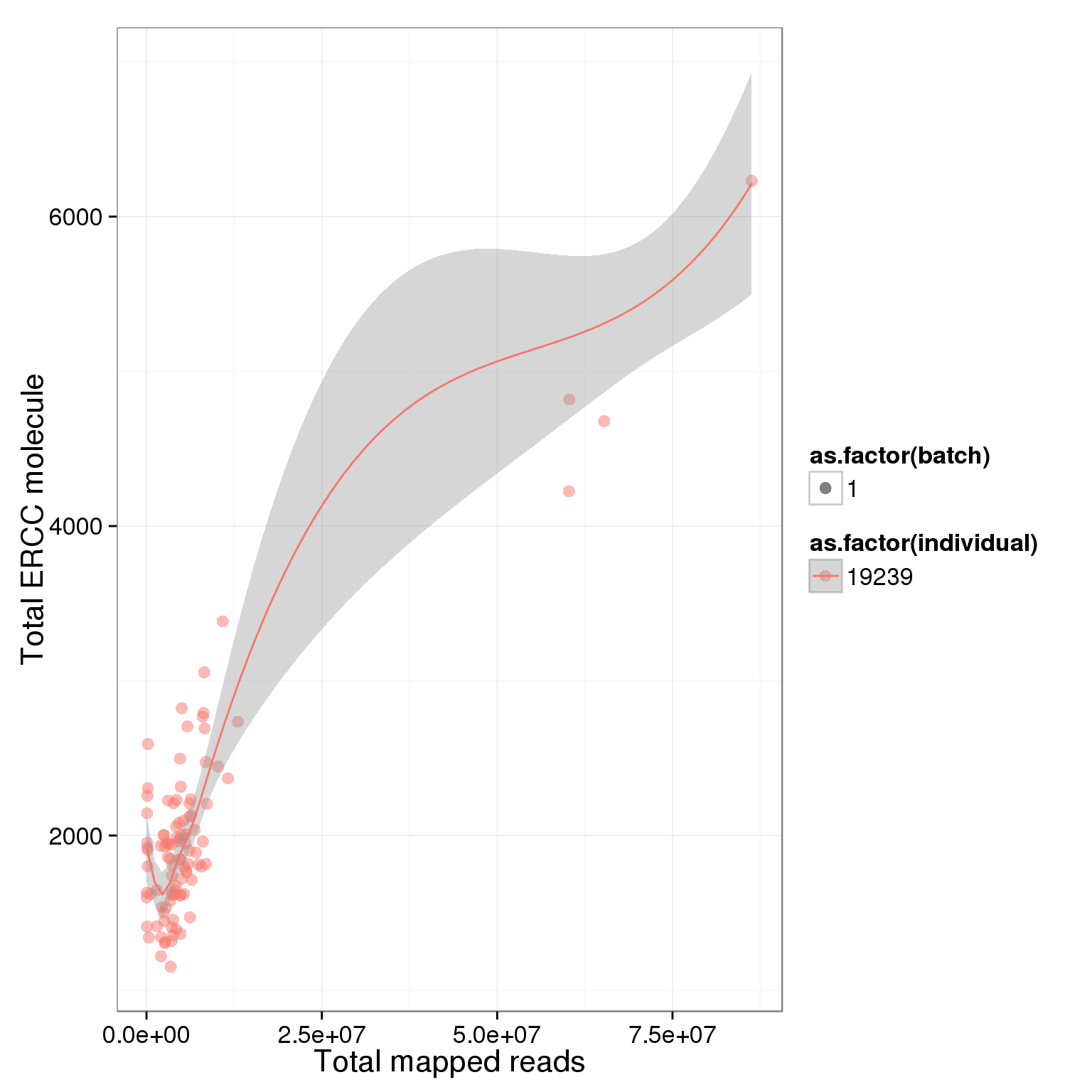
Looking at only the multiplexed single cell libraries (96 samples total, 24 each in lanes 1-4):
# remove the 4 individual cells
summary_per_sample_reads_single <- summary_per_sample_reads[!anno$full_lane, ]

# many plots
ggplot(summary_per_sample_reads_single, aes(x = total.mapped, y = unmapped.ratios, col = as.factor(individual), shape = as.factor(batch))) + geom_point(size = 3, alpha = 0.5) + xlab("Number of mapped reads") + ylab("Umapped reads ratio") + theme(axis.text.x = element_text(angle = 90, hjust = 0.9, vjust = 0.5))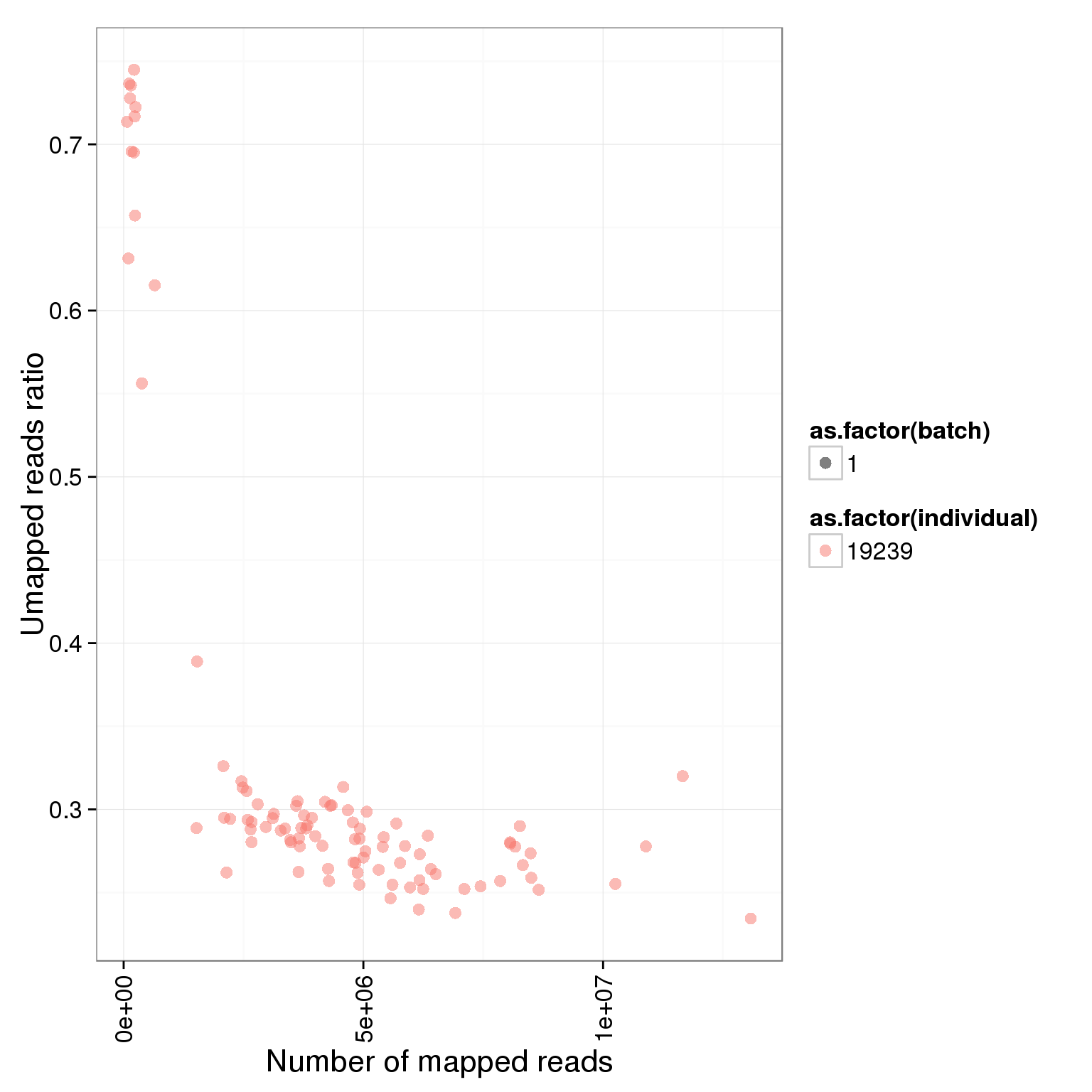
ggplot(summary_per_sample_reads_single, aes(x = total.mapped, y = ERCC.ratios, col = as.factor(individual), shape = as.factor(batch))) + geom_point(size = 3, alpha = 0.5) + xlab("Number of mapped reads") + ylab("Spike-in reads ratio") + theme(axis.text.x = element_text(angle = 90, hjust = 0.9, vjust = 0.5))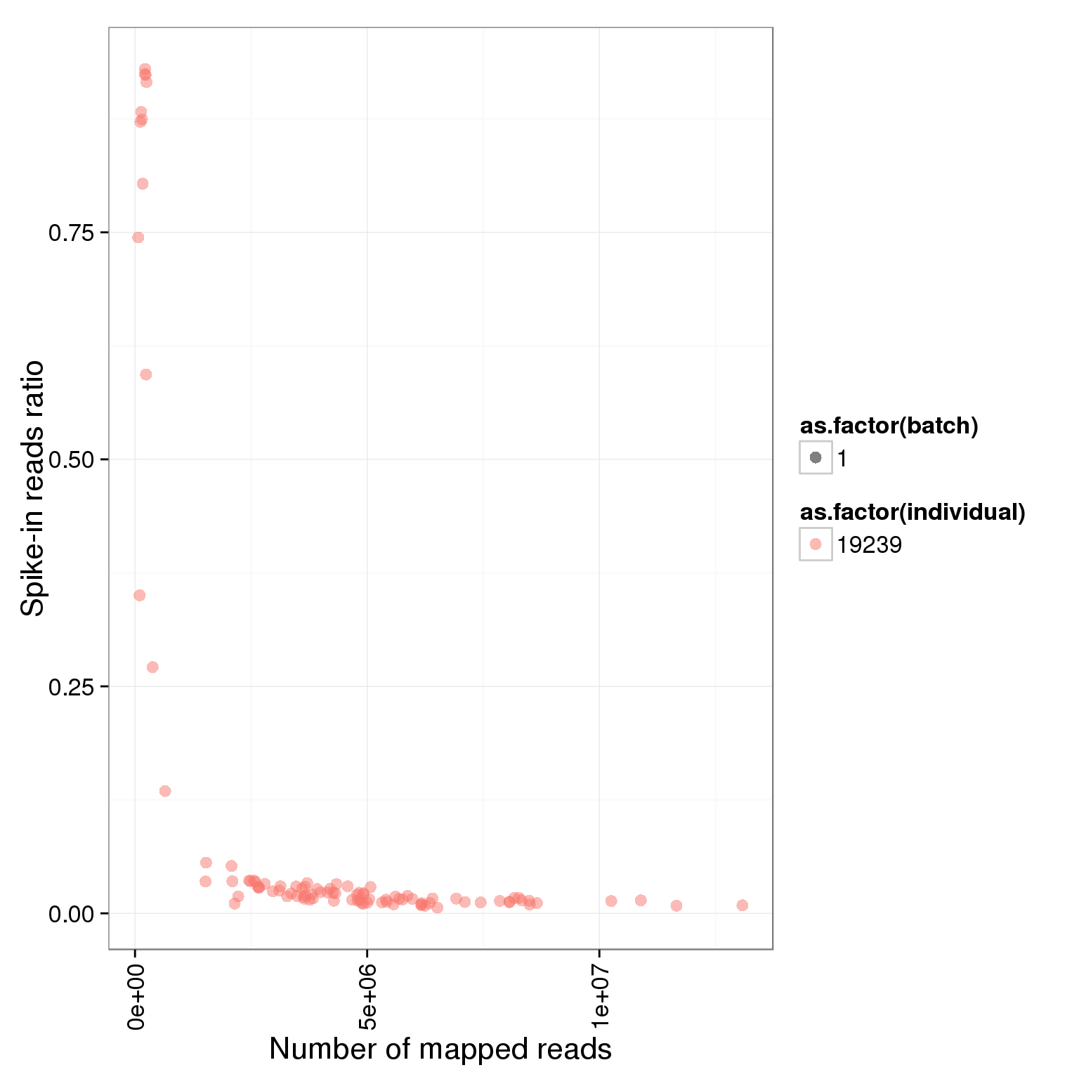
Cell number
The cell number of each capture site is recorded after the cell corting step and before the cells got lysed.
#add cell number per well by merging qc file
summary_per_sample_reads_single_qc <- summary_per_sample_reads_single
summary_per_sample_reads_single_qc$cell_number <- qc$cell.num

ggplot(summary_per_sample_reads_single_qc, aes(x = total.mapped, y = unmapped.ratios, col = as.factor(individual), label = as.character(cell_number))) + geom_text(fontface=3)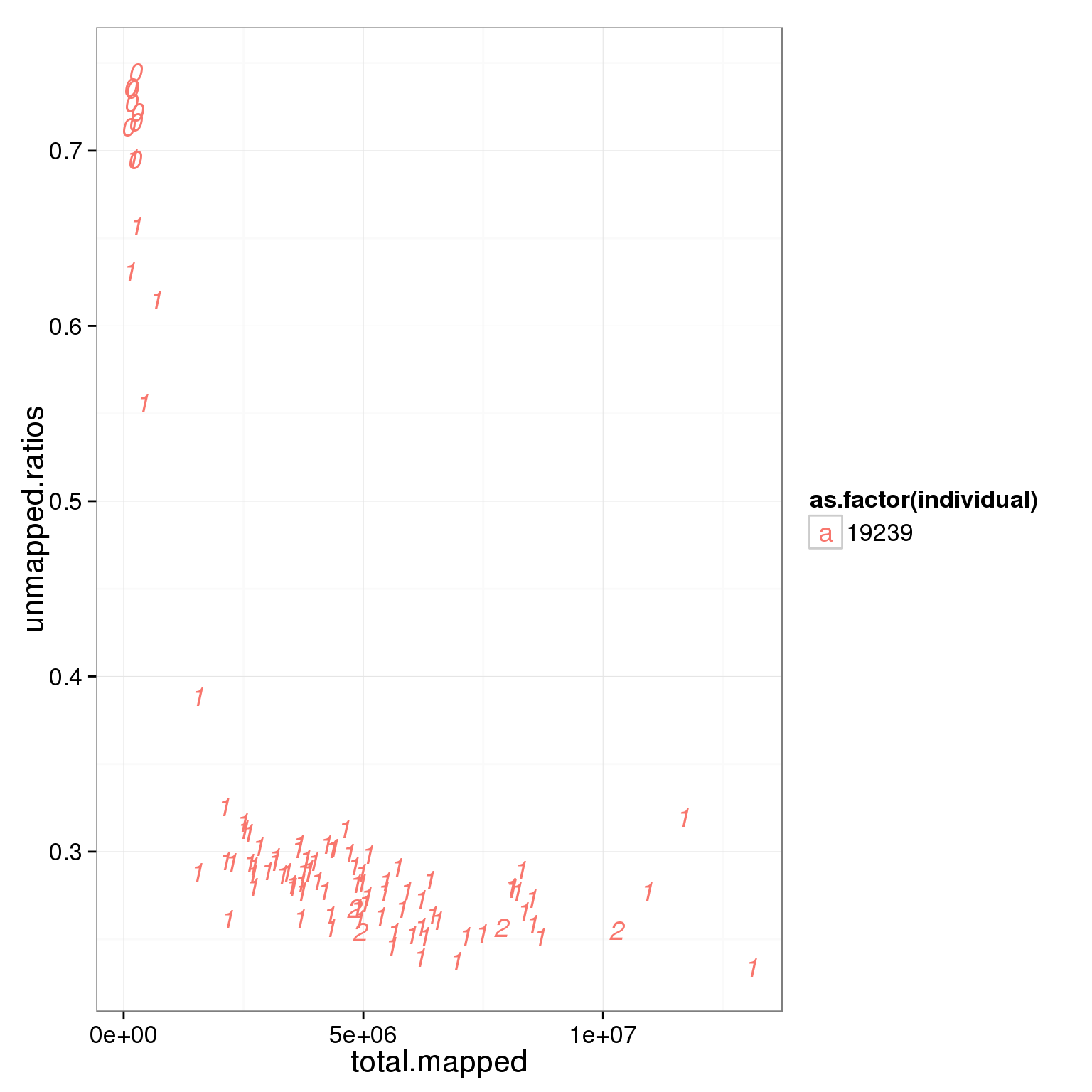
ggplot(summary_per_sample_reads_single_qc, aes(x = total.mapped, y = ERCC.ratios, col = as.factor(individual), label = as.character(cell_number))) + geom_text(fontface=3)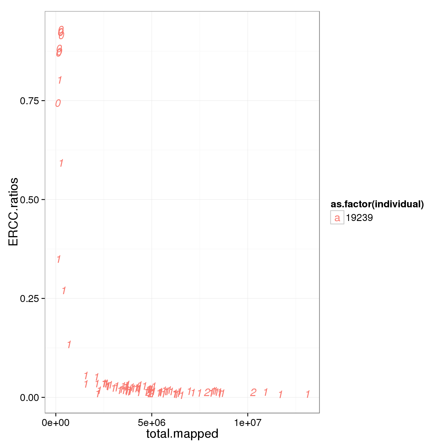
Based on the observation that these is a dinstint cell population with more than 2 million reads, we used it as a cutoff.
#qc filter only keep cells with more than 2 million reads
summary_per_sample_reads_single_qc$qc_filter <- summary_per_sample_reads_single_qc$cell_number == 1 & summary_per_sample_reads_single_qc$total.mapped > 2 * 10^6

ggplot(summary_per_sample_reads_single_qc, aes(x = total.mapped, y = unmapped.ratios, col = qc_filter, label = as.character(cell_number))) + geom_text(fontface=3) + facet_grid(individual ~ batch) + theme(axis.text.x = element_text(angle = 90, hjust = 0.9, vjust = 0.5)) + xlab("Number of mapped reads") + ylab("Umapped reads ratio")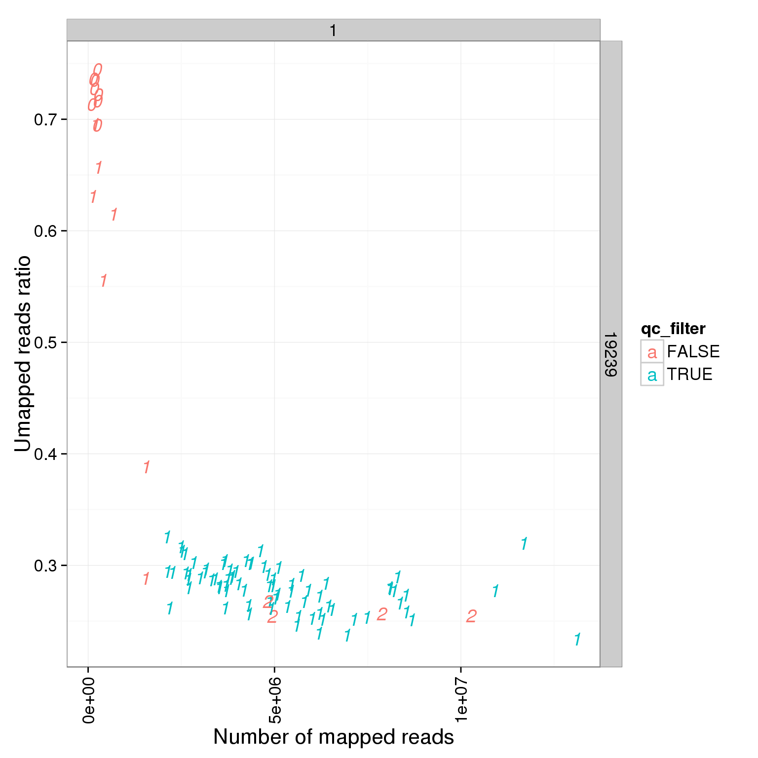
ggplot(summary_per_sample_reads_single_qc, aes(x = total.mapped, y = ERCC.ratios, col = qc_filter, label = as.character(cell_number))) + geom_text(fontface=3) + facet_grid(individual ~ batch) + theme(axis.text.x = element_text(angle = 90, hjust = 0.9, vjust = 0.5)) + xlab("Number of mapped reads") + ylab("Spike-in reads ratio")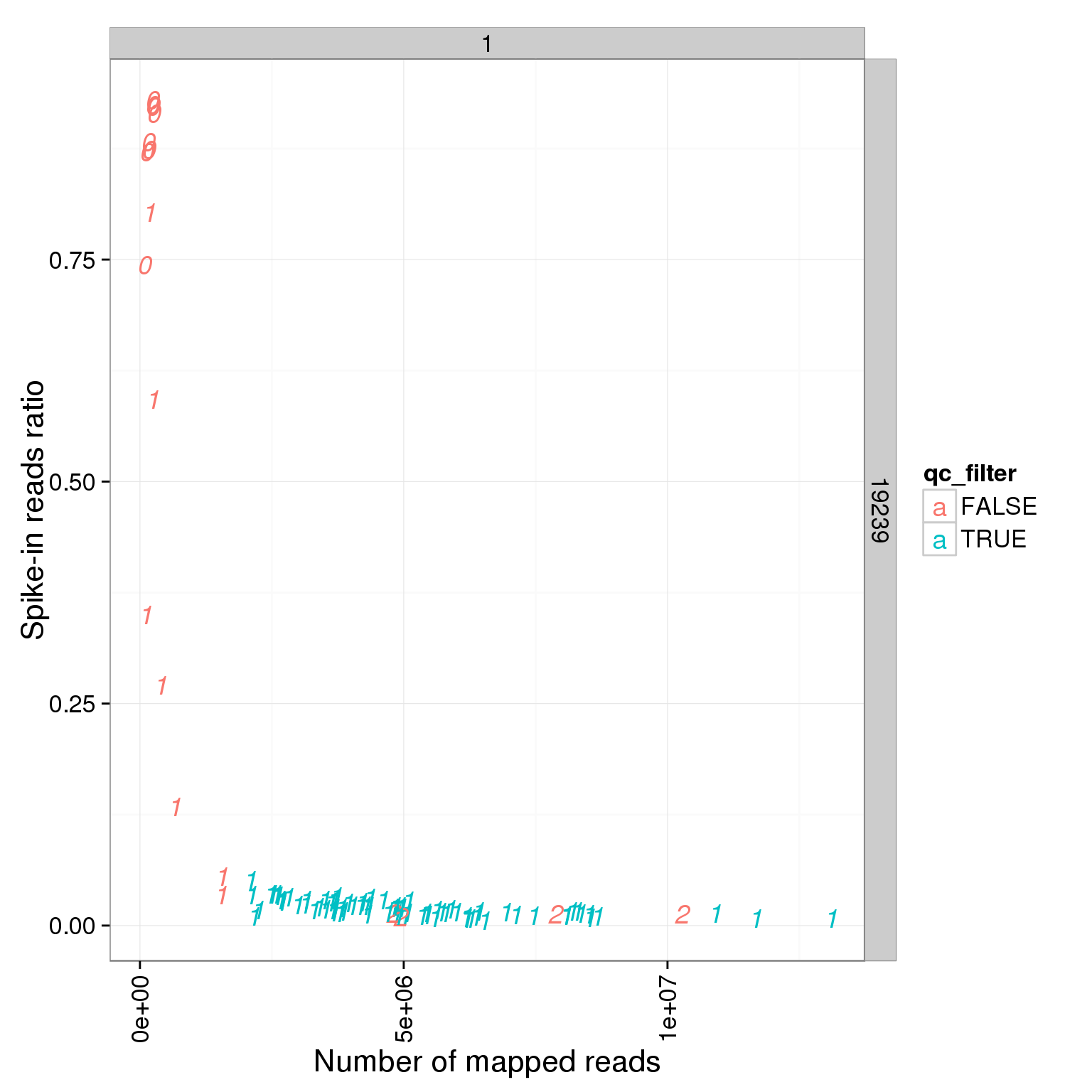
Number of genes detected
Number of genes deteced in LCLS are smaller than iPSCs!!!
## remove genes with no read
expressed <- rowSums(reads) > 0
reads <- reads[expressed, ]
dim(reads)
[1] 13721 100## number of expressed gene in each cell
reads_single <- reads[, anno$full_lane == "FALSE"]
reads_single_gene_number <- colSums(reads_single > 1)
summary_per_sample_reads_single_qc$reads_single_gene_number <- reads_single_gene_number
ggplot(summary_per_sample_reads_single_qc, aes(x = total.mapped, y = reads_single_gene_number, col = qc_filter, label = as.character(cell_number))) + geom_text(fontface=3) + facet_grid(individual ~ batch) + theme(axis.text.x = element_text(angle = 90, hjust = 0.9, vjust = 0.5)) + xlab("Number of mapped reads") + ylab("Number of genes")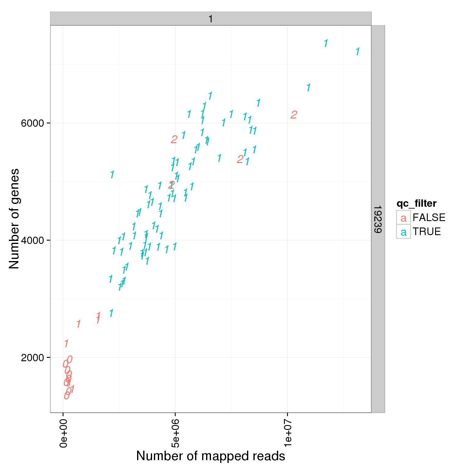
ggplot(summary_per_sample_reads_single_qc, aes(x = reads_single_gene_number, y = ERCC.ratios, col = qc_filter, label = as.character(cell_number))) + geom_text(fontface=3) + facet_grid(individual ~ batch) + theme(axis.text.x = element_text(angle = 90, hjust = 0.9, vjust = 0.5)) + xlab("Number of genes") + ylab("Spike-in reads ratio")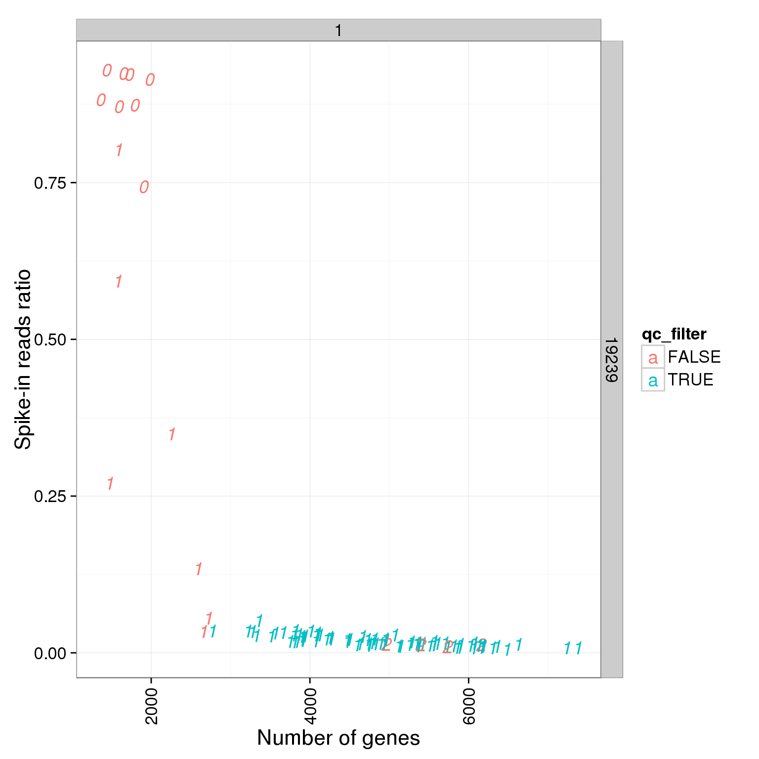
What are the numbers of detected genes of the 4 heavily-sequenced individual cells?
## the 4 individual cells
reads_4 <- reads[, anno$full_lane == "TRUE"]
reads_4_gene_number <- colSums(reads_4 > 1)
reads_4_gene_number
NA19239.1.A9E1 NA19239.1.B2E2 NA19239.1.B4H1 NA19239.1.D2H2
5896 6911 6025 5783 Reads mapped to mitochondrial genes
## create a list of mitochondrial genes (13 protein-coding genes)
## MT-ATP6, MT-CYB, MT-ND1, MT-ND4, MT-ND4L, MT-ND5, MT-ND6, MT-CO2, MT-CO1, MT-ND2, MT-ATP8, MT-CO3, MT-ND3
mtgene <- c("ENSG00000198899", "ENSG00000198727", "ENSG00000198888", "ENSG00000198886", "ENSG00000212907", "ENSG00000198786", "ENSG00000198695", "ENSG00000198712", "ENSG00000198804", "ENSG00000198763","ENSG00000228253", "ENSG00000198938", "ENSG00000198840")

## reads of mt genes in single cells
mt_reads <- reads_single[mtgene,]
dim(mt_reads)
[1] 13 96## mt ratio of single cell
mt_reads_total <- apply(mt_reads, 2, sum)
summary_per_sample_reads_single_qc$mt_reads_total <- mt_reads_total
summary_per_sample_reads_single_qc$mt_reads_ratio <- summary_per_sample_reads_single_qc$mt_reads_total/summary_per_sample_reads_single_qc$total.mapped
ggplot(summary_per_sample_reads_single_qc, aes(x = total.mapped, y = mt_reads_ratio, col = qc_filter, label = as.character(cell_number))) + geom_text(fontface=3) + facet_grid(individual ~ batch) + theme(axis.text.x = element_text(angle = 90, hjust = 0.9, vjust = 0.5)) + xlab("Number of mapped reads") + ylab("Mitochondrial ratio")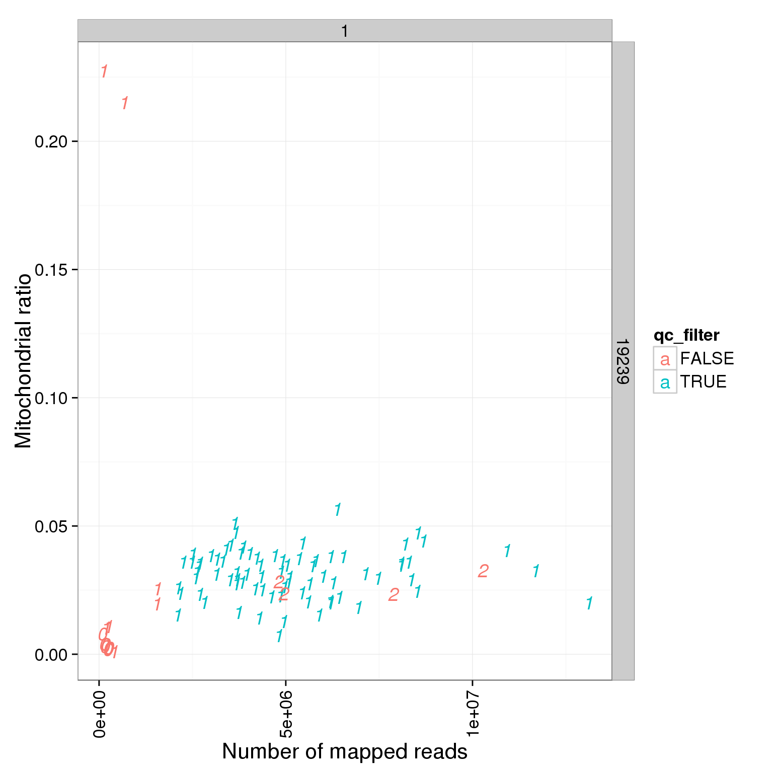
ggplot(summary_per_sample_reads_single_qc, aes(x = mt_reads_ratio, y = ERCC.ratios, col = qc_filter, label = as.character(cell_number))) + geom_text(fontface=3) + facet_grid(individual ~ batch) + theme(axis.text.x = element_text(angle = 90, hjust = 0.9, vjust = 0.5)) + xlab("Mitochondrial ratio") + ylab("Spike-in reads ratio")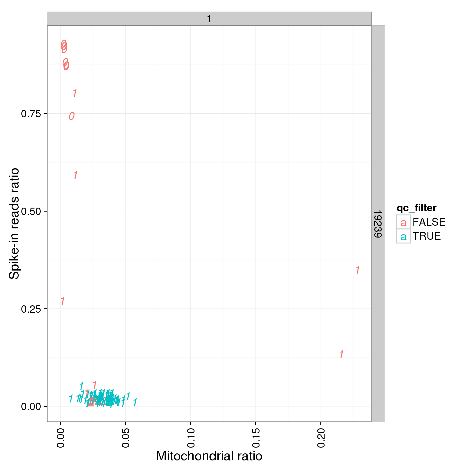
ggplot(summary_per_sample_reads_single_qc, aes(x = reads_single_gene_number, y = mt_reads_ratio, col = qc_filter, label = as.character(cell_number))) + geom_text(fontface=3) + facet_grid(individual ~ batch) + theme(axis.text.x = element_text(angle = 90, hjust = 0.9, vjust = 0.5)) + xlab("Number of genes") + ylab("Mitochondrial ratio")
PCA
Calculate the counts per million for the singe cells.
reads_cells <- reads_single
reads_cells_cpm <- cpm(reads_cells)
Select the most variable genes.
reads_cells_cpm_log_var <- log(apply(reads_cells_cpm, 1, var))
hist(reads_cells_cpm_log_var)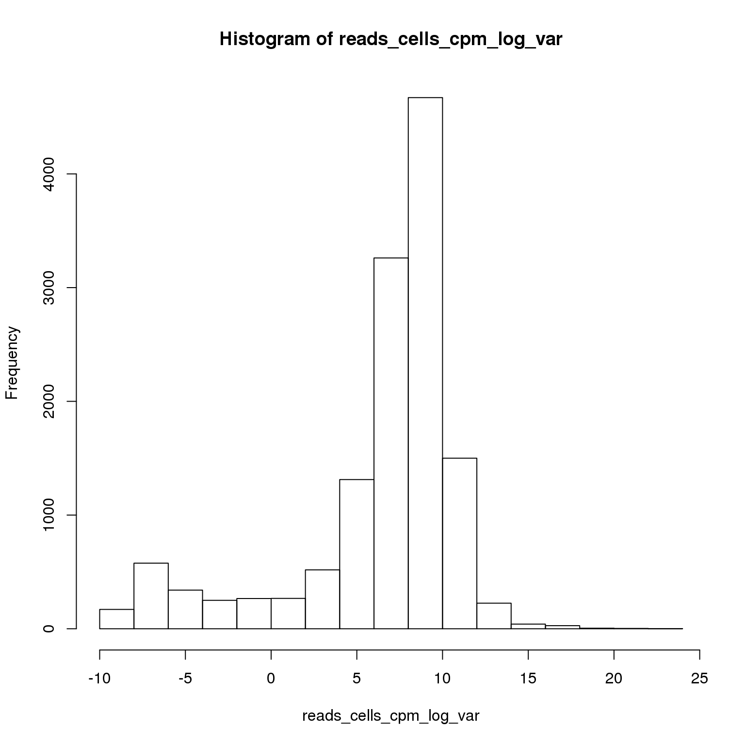
sum(reads_cells_cpm_log_var > 8)[1] 6473Using the 6473 most variable genes, perform PCA.
reads_cells_cpm <- reads_cells_cpm[reads_cells_cpm_log_var > 8, ]
pca_reads_cells <- prcomp(t(reads_cells_cpm), retx = TRUE, scale. = TRUE,
                          center = TRUE)
plot(pca_reads_cells)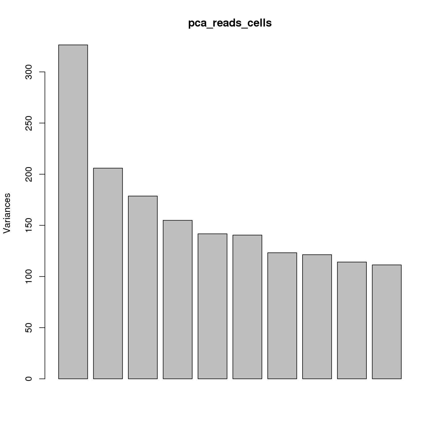
pca_reads_cells$perc_explained <- pca_reads_cells$sdev^2 / sum(pca_reads_cells$sdev^2) * 100
plot(pca_reads_cells$perc_explained)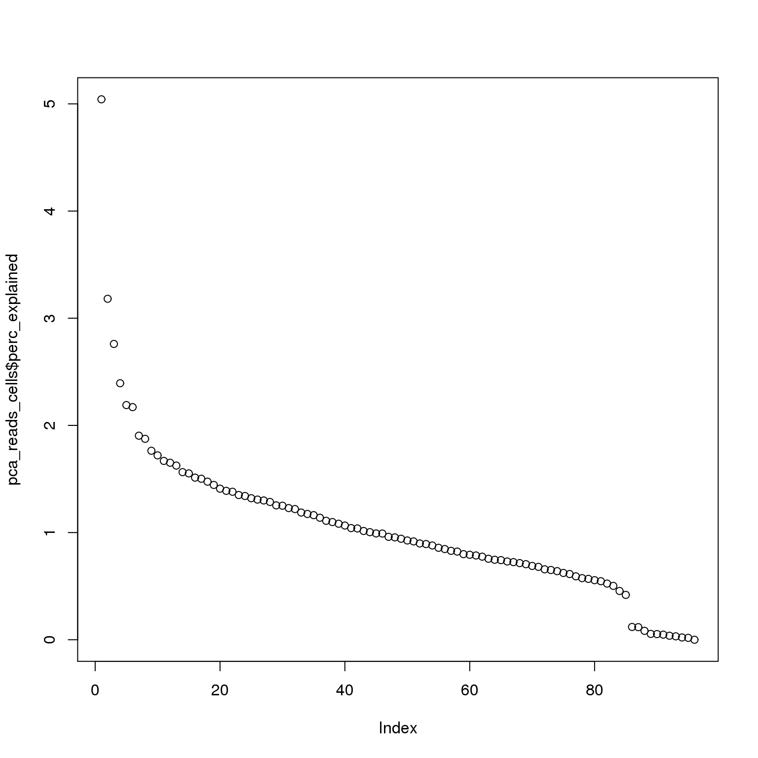
The first PC accounts for 5% of the variance and the second PC 3%.
stopifnot(colnames(reads_cells) ==
            paste(paste0("NA", summary_per_sample_reads_single_qc$individual),
                   summary_per_sample_reads_single_qc$batch,
                   summary_per_sample_reads_single_qc$well, sep = "."))
pca_reads_cells_anno <- cbind(summary_per_sample_reads_single_qc, pca_reads_cells$x)
ggplot(pca_reads_cells_anno, aes(x = PC1, y = PC2, col = as.factor(individual),
shape = as.factor(batch))) +
geom_point()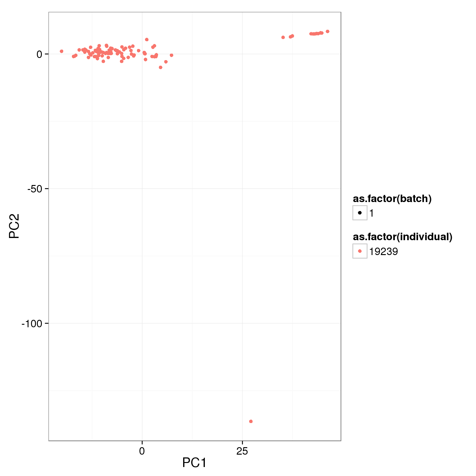
Cutoffs
Using various simple filtering cutoffs.
pca_reads_cells_anno$cell_filter <- pca_reads_cells_anno$cell_number == 1
ggplot(pca_reads_cells_anno, aes(x = PC1, y = PC2, col = cell_filter)) +
  geom_point()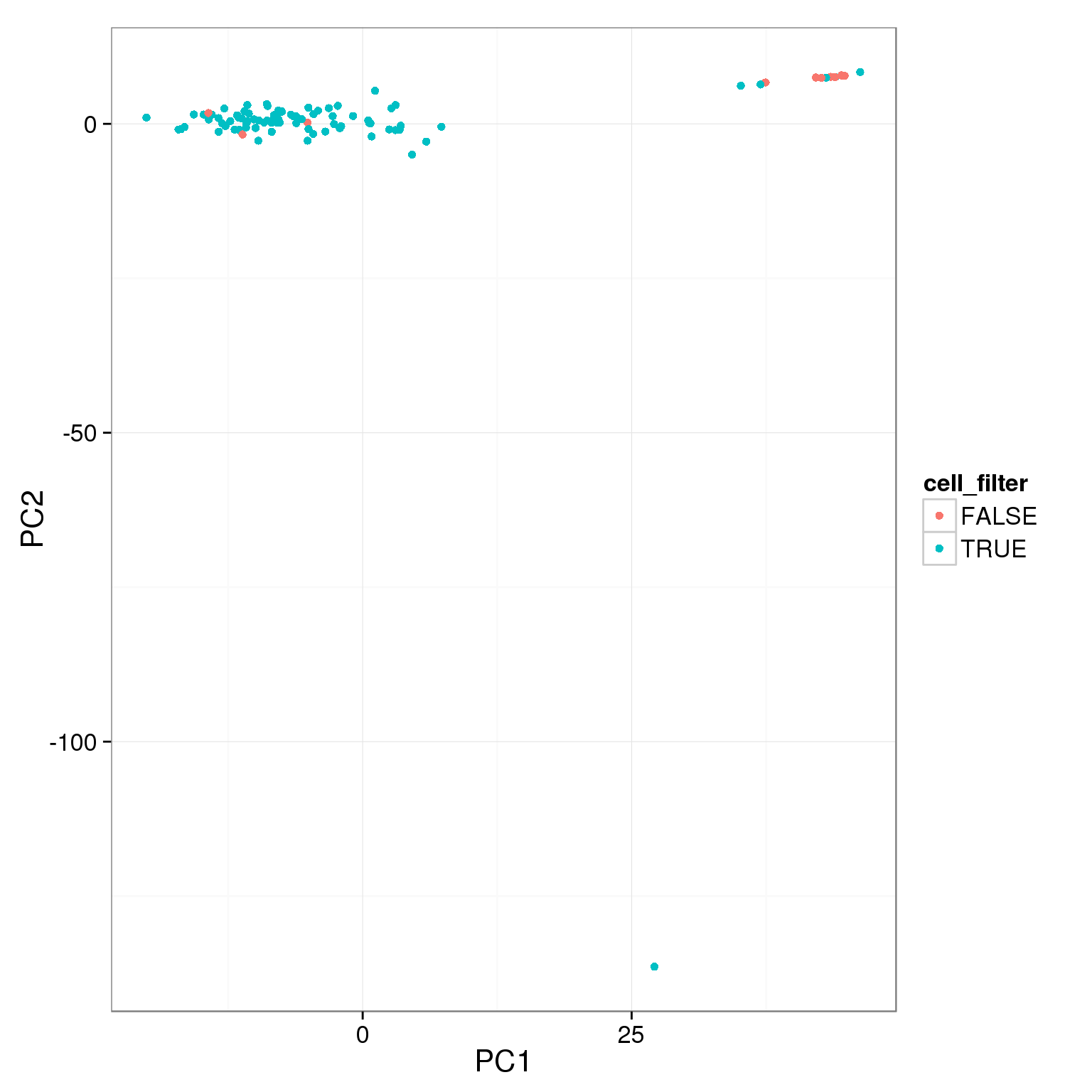
pca_reads_cells_anno$total_cutoff <- pca_reads_cells_anno$total.mapped > 1.5 * 10^6
ggplot(pca_reads_cells_anno, aes(x = PC1, y = PC2, col = total_cutoff)) +
  geom_point()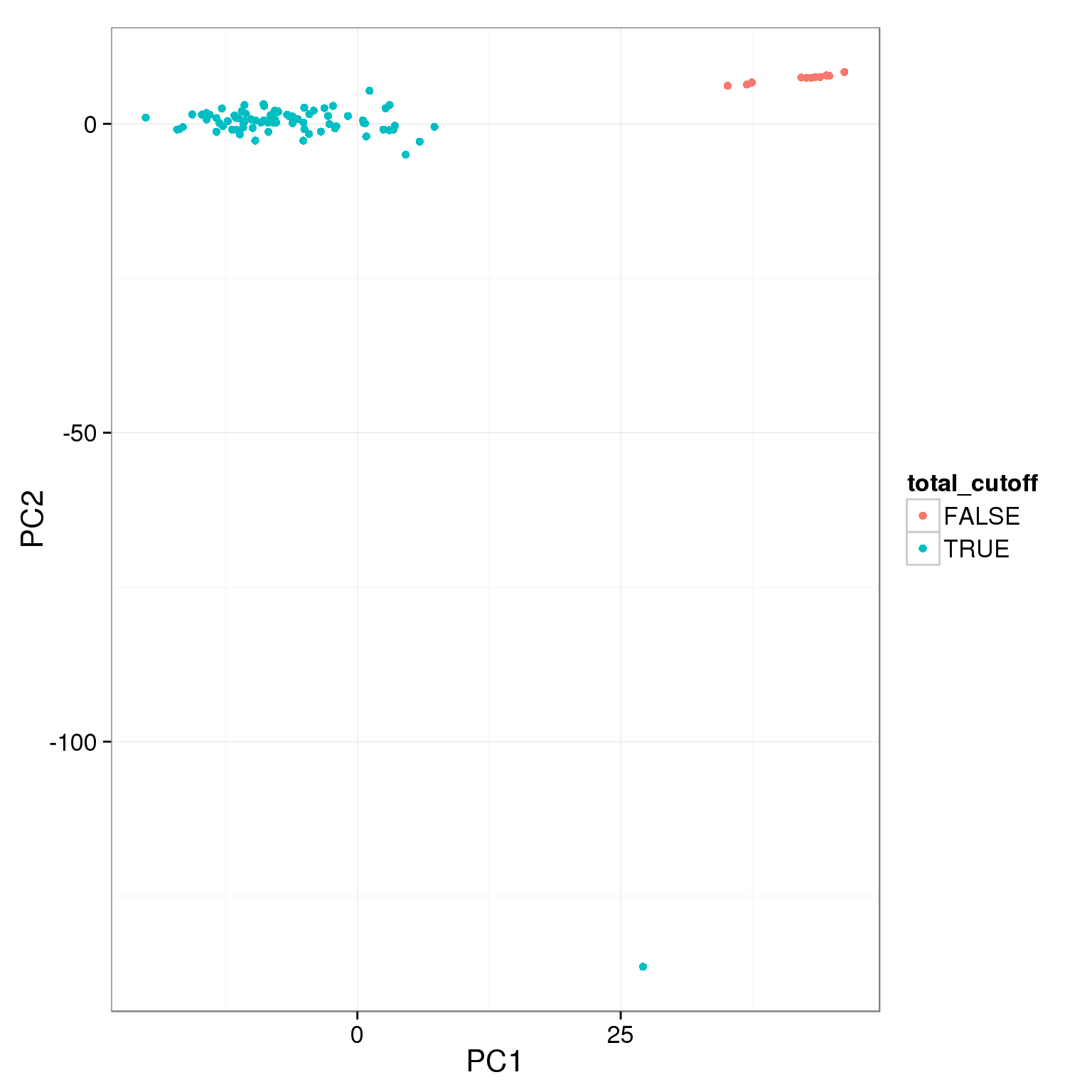
pca_reads_cells_anno$unmapped_cutoff <- pca_reads_cells_anno$unmapped.ratios < 0.4
ggplot(pca_reads_cells_anno, aes(x = PC1, y = PC2, col = unmapped_cutoff)) +
  geom_point()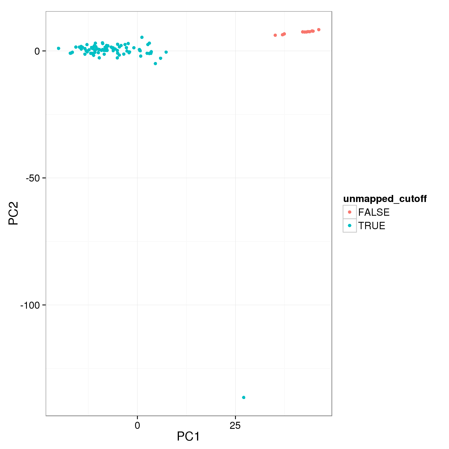
pca_reads_cells_anno$ERCC_cutoff <- pca_reads_cells_anno$ERCC.ratios < 0.05
ggplot(pca_reads_cells_anno, aes(x = PC1, y = PC2, col = ERCC_cutoff)) +
  geom_point()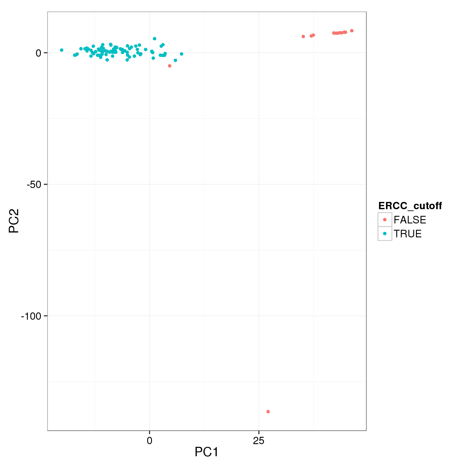
pca_reads_cells_anno$gene_filter <- pca_reads_cells_anno$reads_single_gene_number  > 3000
ggplot(pca_reads_cells_anno, aes(x = PC1, y = PC2, col = gene_filter)) +
  geom_point()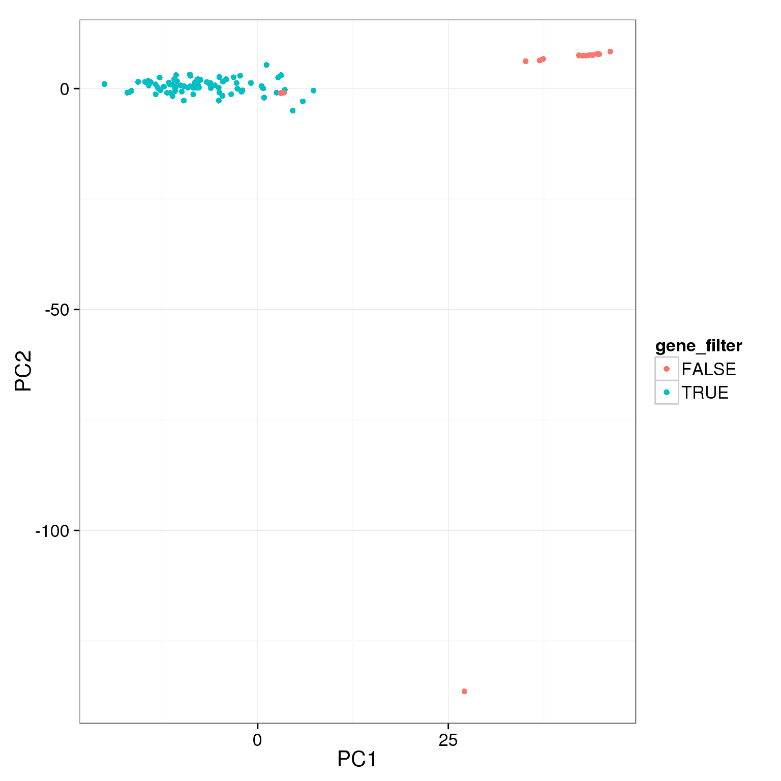
pca_reads_cells_anno$mt_filter <- pca_reads_cells_anno$mt_reads_ratio < 0.15
ggplot(pca_reads_cells_anno, aes(x = PC1, y = PC2, col = mt_filter)) +
  geom_point()
The two cutoffs, total reads and cell number, largely overlap.
table(pca_reads_cells_anno$cell_filter, pca_reads_cells_anno$total_cutoff,
      dnn = c("Num cells == 1", "Total reads > 1.5e6"))
Total reads > 1.5e6
Num cells == 1 FALSE TRUE
FALSE 8 4
TRUE 5 79Add the third cutoff, 3000 genes
pca_reads_cells_anno$qc_filter <- pca_reads_cells_anno$total_cutoff &
                                  pca_reads_cells_anno$gene_filter &
                                  pca_reads_cells_anno$cell_filter

ggplot(pca_reads_cells_anno, aes(x = PC1, y = PC2, col = qc_filter,
                                 label = as.character(cell_number))) +
  geom_text(fontface=3)
Apply all the cutoffs
pca_reads_cells_anno$qc_filter_all <- pca_reads_cells_anno$cell_filter &
                                      pca_reads_cells_anno$total_cutoff &
                                      pca_reads_cells_anno$unmapped_cutoff &
                                      pca_reads_cells_anno$ERCC_cutoff &
                                      pca_reads_cells_anno$gene_filter &
                                      pca_reads_cells_anno$mt_filter

ggplot(pca_reads_cells_anno, aes(x = PC1, y = PC2, col = qc_filter_all,
                                 label = as.character(cell_number))) +
  geom_text(fontface=3)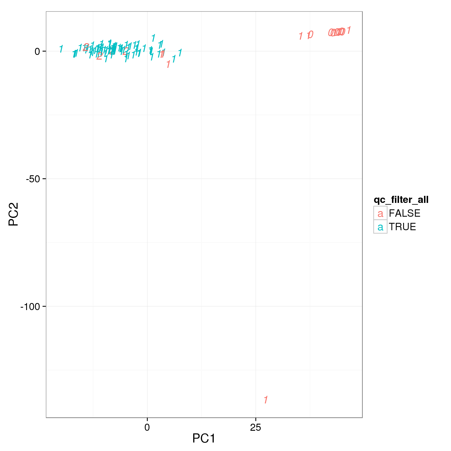
How many cells do we keep from each individual and batch using this filter?
table(pca_reads_cells_anno[pca_reads_cells_anno$qc_filter,
                           c("individual", "batch")])
batch
individual 1
19239 76table(pca_reads_cells_anno[pca_reads_cells_anno$qc_filter_all,
c("individual", "batch")]) batch
individual 1
19239 75Output list of single cells to keep.
stopifnot(nrow(pca_reads_cells_anno) == nrow(anno[anno$full_lane == "FALSE", ]))
quality_single_cells <- anno %>%
  filter(full_lane == "FALSE") %>%
  filter(pca_reads_cells_anno$qc_filter_all) %>%
  select(sample_id)
stopifnot(!grepl("TRUE", quality_single_cells$sample_id))
write.table(quality_single_cells,
            file = "../data/quality-single-cells-lcl.txt", quote = FALSE,
            sep = "\t", row.names = FALSE, col.names = FALSE)
Session information
sessionInfo()R version 3.2.0 (2015-04-16)
Platform: x86_64-unknown-linux-gnu (64-bit)
locale:
[1] LC_CTYPE=en_US.UTF-8 LC_NUMERIC=C
[3] LC_TIME=en_US.UTF-8 LC_COLLATE=en_US.UTF-8
[5] LC_MONETARY=en_US.UTF-8 LC_MESSAGES=en_US.UTF-8
[7] LC_PAPER=en_US.UTF-8 LC_NAME=C
[9] LC_ADDRESS=C LC_TELEPHONE=C
[11] LC_MEASUREMENT=en_US.UTF-8 LC_IDENTIFICATION=C
attached base packages:
[1] stats graphics grDevices utils datasets methods base
other attached packages:
[1] edgeR_3.10.2 limma_3.24.9 ggplot2_1.0.1 dplyr_0.4.1 knitr_1.10.5
loaded via a namespace (and not attached):
[1] Rcpp_0.11.6 magrittr_1.5 MASS_7.3-40 munsell_0.4.2
[5] colorspace_1.2-6 stringr_1.0.0 plyr_1.8.2 tools_3.2.0
[9] parallel_3.2.0 grid_3.2.0 gtable_0.1.2 DBI_0.3.1
[13] htmltools_0.2.6 lazyeval_0.1.10 yaml_2.1.13 assertthat_0.1
[17] digest_0.6.8 reshape2_1.4.1 formatR_1.2 evaluate_0.7
[21] rmarkdown_0.6.1 labeling_0.3 stringi_0.4-1 scales_0.2.4
[25] proto_0.3-10