Final LCL subsampling plots

Input

library("dplyr")
library("tidyr")
library("ggplot2")
library("cowplot")
theme_set(theme_bw(base_size = 16))
theme_update(panel.grid.minor.x = element_blank(),
             panel.grid.minor.y = element_blank(),
             panel.grid.major.x = element_blank(),
             panel.grid.major.y = element_blank())

The subsampling statistics were generated with subsample-pipeline.py and detect-genes.R.

d <- read.table("../data/subsampling-results-lcl.txt",
                header = TRUE, sep = "\t", stringsAsFactors = FALSE)
d$depth_mil <- d$depth / 10^6
d$counts_thous <- d$counts / 10^3
d$counts_mil <- d$counts / 10^6
str(d)

'data.frame':   144 obs. of  11 variables:
 $ depth       : int  1000000 1000000 1000000 1000000 1000000 1000000 1000000 1000000 10000000 10000000 ...
 $ type        : chr  "molecules" "reads" "molecules" "reads" ...
 $ well        : chr  "A9E1" "A9E1" "B2E2" "B2E2" ...
 $ gene_subset : chr  "ENSG" "ENSG" "ENSG" "ENSG" ...
 $ num_cells   : int  1 1 1 1 1 1 1 1 1 1 ...
 $ seed        : int  1 1 1 1 1 1 1 1 1 1 ...
 $ genes       : int  5290 5290 6253 6254 5319 5319 4925 4925 6605 6606 ...
 $ counts      : num  21630 493812 30932 518453 19398 ...
 $ depth_mil   : num  1 1 1 1 1 1 1 1 10 10 ...
 $ counts_thous: num  21.6 493.8 30.9 518.5 19.4 ...
 $ counts_mil  : num  0.0216 0.4938 0.0309 0.5185 0.0194 ...

Endogenous genes detected

p_genes_ensg <- ggplot(d[d$gene_subset == "ENSG" &
                         d$type == "molecules", ],
                       aes(x = as.factor(depth_mil), y = genes)) +
  geom_boxplot() + 
  geom_point(aes(color  = well)) +
  scale_color_brewer(palette = "Dark2", name = "Single cell") +
  theme(legend.position = "none") +
  labs(x = expression("Sequencing depth (" * 10^6 * ")"),
       y = "Genes detected",
       title = "Endogenous genes")
p_genes_ensg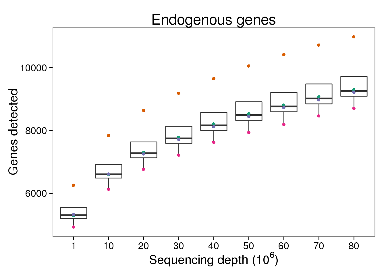

ERCC control genes detected

p_genes_ercc <- p_genes_ensg %+% d[d$gene_subset == "ERCC" &
                                   d$type == "molecules", ] +
  labs(title = "ERCC controls")
p_genes_ercc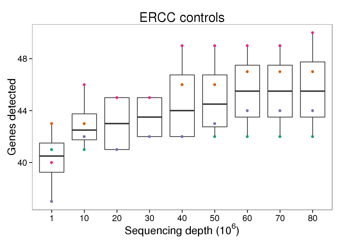

Endogenous molecules

p_molecules_ensg <- p_genes_ensg %+% d[d$type == "molecules" &
                                       d$gene_subset == "ENSG", ] %+%
  aes(y = counts_thous) +
  labs(y = expression("Molecules (" * 10^3 * ")"))
p_molecules_ensg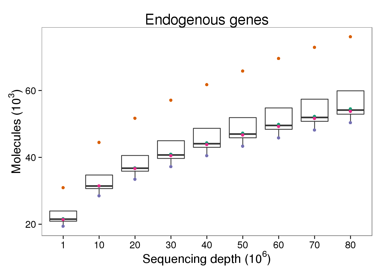

ERCC molecules

p_molecules_ercc <- p_molecules_ensg %+% d[d$type == "molecules" &
                                           d$gene_subset == "ERCC", ] +
  labs(title = "ERCC controls") +
  theme(legend.position = c(0.75, 0.35))
p_molecules_ercc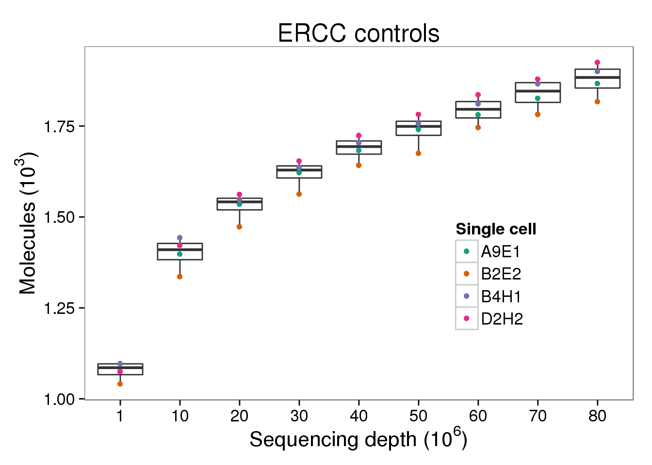

Endogenous reads

p_reads_ensg <- p_molecules_ensg %+% d[d$type == "reads" &
                                       d$gene_subset == "ENSG", ] +
  aes(y = counts_mil) +
  labs(y = expression("Reads (" * 10^6 * ")"))
p_reads_ensg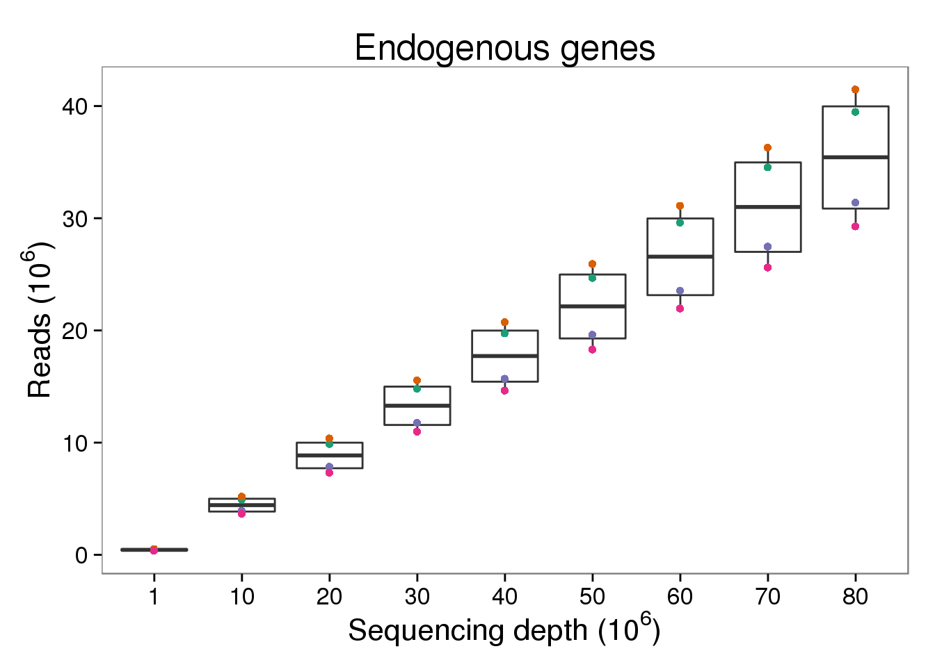

ERCC reads

p_reads_ercc <- p_reads_ensg %+% d[d$type == "reads" &
                                   d$gene_subset == "ERCC", ] +
  labs(title = "ERCC controls")
p_reads_ercc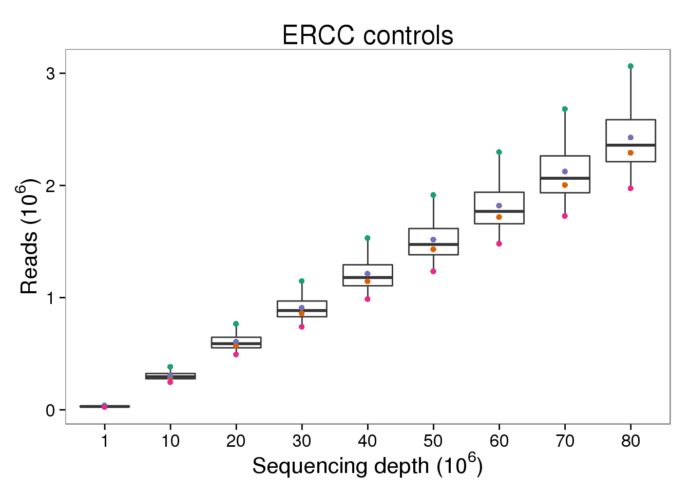

Final plot for supplementary figure

plot_final <- plot_grid(p_genes_ensg, p_genes_ercc,
                        p_molecules_ensg, p_molecules_ercc,
                        p_reads_ensg, p_reads_ercc,
                        ncol = 2, labels = LETTERS[1:6])
png("../paper/figure/fig-subsample-lcl.png", width = 8, height = 12,
    units = "in", res = 300)
plot_final
dev.off()

png 
  2 

Session information

sessionInfo()

R version 3.2.0 (2015-04-16)
Platform: x86_64-unknown-linux-gnu (64-bit)

locale:
 [1] LC_CTYPE=en_US.UTF-8       LC_NUMERIC=C              
 [3] LC_TIME=en_US.UTF-8        LC_COLLATE=en_US.UTF-8    
 [5] LC_MONETARY=en_US.UTF-8    LC_MESSAGES=en_US.UTF-8   
 [7] LC_PAPER=en_US.UTF-8       LC_NAME=C                 
 [9] LC_ADDRESS=C               LC_TELEPHONE=C            
[11] LC_MEASUREMENT=en_US.UTF-8 LC_IDENTIFICATION=C       

attached base packages:
[1] stats     graphics  grDevices utils     datasets  methods   base     

other attached packages:
[1] cowplot_0.3.1 ggplot2_1.0.1 tidyr_0.2.0   dplyr_0.4.2   knitr_1.10.5 

loaded via a namespace (and not attached):
 [1] Rcpp_0.12.4        magrittr_1.5       MASS_7.3-40       
 [4] munsell_0.4.3      colorspace_1.2-6   R6_2.1.1          
 [7] stringr_1.0.0      httr_0.6.1         plyr_1.8.3        
[10] tools_3.2.0        parallel_3.2.0     grid_3.2.0        
[13] gtable_0.1.2       DBI_0.3.1          htmltools_0.2.6   
[16] yaml_2.1.13        assertthat_0.1     digest_0.6.8      
[19] RColorBrewer_1.1-2 reshape2_1.4.1     formatR_1.2       
[22] bitops_1.0-6       RCurl_1.95-4.6     evaluate_0.7      
[25] rmarkdown_0.6.1    labeling_0.3       stringi_1.0-1     
[28] scales_0.4.0       proto_0.3-10