BASiCS analysis of Mouse ESC dataset

Introduction
Data pre-processing
Effect of sequencing depth on total molecule counts
Session information

Last updated: 2015-10-01

Code version: 0a8ae478de84ce46ed5572c0b2b85e3337f3f71c

The first half of the analysis is the data cleaning steps performed in Vallejos et al., 2015 to reproduce the steps performed in Islam et al., 2014. In the second half I compare the total molecule counts from this clean data to the sequencing depth per sample to determine if there is still a relationship between sequencing depth and total molecule count.

Introduction

This document shows the code used when illustrating the use of BASiCS by analysing the mouse ESC dataset described in Islam et al (2014)¹. To start the analysis, the following data must be dowloaded and stored in data.path directory.

Expression counts. File ‘GSE46980_CombinedMoleculeCounts.tab’ from Series GSE46980.
Quality control information. File ‘187_3lanes_CA.txt’ (provided by Sten Linnarson).
Input molecules of spike-in genes. File ‘SilverBulletCTRLConc.txt’ (provided by Sten Linnarson).
List of highly variable genes detected by Islam et al (2014). Supplementary Table 1 (noisy genes) in Islam et al (2014)

# Here, we stored the 3 files mentioned above in the current R working directory
# Change this path as necessary

#setwd("/Users/catalinavallejos/Documents/MRC/Projects/SCE/LaTeX/BASiCS/AnalysisMouseESC/")
# data.path = getwd()
data.path = "/mnt/gluster/home/jdblischak/basics/AnalysisMouseESC"

In addition, the following libraries must be loaded before performing the analysis

#################################
# REQUIRED LIBRARIES ############
#################################
library(BASiCS) # To perform BASiCS analysis
# Please ignore the message 'No methods found in "BiocGenerics" for requests: displayTechIndicator, displaySpikeInput'
# BASiCS only needs to import the generic functions, not the associated methods. 

#################################
# OPTIONAL LIBRARIES ############
#################################
library(data.table) # For fast pre-processing of large datasets. Can be replaced by standard 'data.frame' objects

Data pre-processing

Loading the expression counts

# Matrix of expression counts (ignoring metadata)
Counts <- fread(paste0(data.path,"/GSE46980_CombinedMoleculeCounts.tab"),skip=6,drop=c("Chr","Pos","Strand","TrLen","MinExonHits","ExonHits"))
Cells <- as.vector(t(read.table(paste0(data.path,"/GSE46980_CombinedMoleculeCounts.tab"),skip=5, nrows = 1, header = F)[-1]))
SpikesInfo <- fread(paste0(data.path,"/SilverBulletCTRLConc.txt"), select=c("ERCC_ID","Name","molecules_in_each_chamber"))

Counts is the matrix of expression counts. The first column in Counts contains the identifiers for each of the 25914 transcripts and the remaining columns contain the observed expression counts for each of the 96 cells in the sample.
Cells contains cell identifiers for each of the 96 cells in the sample. These identifiers are required in order to combine the quality control information.
SpikesInfo contains the input molecules that were added to the cell’s lysis (for each of the 92 spike-in genes)

The first step is to fix the format of genes and cells’ identifiers:

# Cell identifiers
setnames(Counts,names(Counts),c("Name",Cells)) 

# Gene identifiers 
# ERCC identifiers must start with 'ERCC' (required to combine with the information about input molecules)
setkey(Counts,Name); setkey(SpikesInfo,Name)
Counts <- merge(Counts,SpikesInfo,all=TRUE)
# Creating a variable containing gene names (including ERCC names)
Counts$Name <- ifelse(is.na(Counts$ERCC_ID),Counts$Name,Counts$ERCC_ID) 
# Excluding 4 spike-in genes that are not part of the ERCC molecules.
Counts <- Counts[-grep("SPIKE",Counts$Name)] 

# Removing a column which is no longer required
Counts=Counts[,ERCC_ID:=NULL]

Current processed data contains 25910 genes and 96 cells. The next step is to remove those cells that did not pass the quality control criteria employed by Islam et al (2014).

QC_Info <- fread(paste0(data.path,"/187_3lanes_CA.txt"))
GoodCells=QC_Info$Well[QC_Info$GoodCell==1]
# 9 other cells deleted as possible MEF (information provided by Sten Linnarson)
MEF=c("D02", "E02", "A06", "H07", "D08", "A09", "G10", "F12", "G12") 
GoodCells=GoodCells[!(GoodCells %in% MEF)]
Counts <- subset(Counts, select = c("Name",GoodCells,"molecules_in_each_chamber"))

Current processed data contains 25910 genes and 41 cells. The next step is to remove those transcrips that are very lowly expressed.

GenesIDs <- Counts$Name
# Fixing a gene name that was missinterpreted by excel... 
GenesIDs[GenesIDs=="1-Sep"]="Sept1" 
SpikesInput <- Counts$molecules_in_each_chamber
Counts = Counts[, Name := NULL]
Counts = Counts[, molecules_in_each_chamber := NULL]

SumByGene = rowSums(Counts)
GenesInclude = I(SumByGene>=41)
CountsQC = as.matrix(Counts[GenesInclude,]) 
GenesQC.IDs = GenesIDs[GenesInclude]
SpikesInputQC = SpikesInput[GenesInclude]
# Fixing a gene name that was missinterpreted by excel...
GenesQC.IDs[GenesQC.IDs=="1-Sep"]="Sept1" 
# Creating and identifier of spike-in genes
TechQC=ifelse(1:nrow(CountsQC) %in% grep("ERCC",GenesQC.IDs),T,F)

Current processed data contains 7941 genes and 41 cells. Finally, we need to re-arrange the data such that the expression counts are at the bottom of the table.

CountsQC=rbind(CountsQC[!TechQC,],CountsQC[TechQC,])
GenesQC.IDs=c(GenesQC.IDs[!TechQC],GenesQC.IDs[TechQC])
SpikesInputQC = c(SpikesInputQC[!TechQC],SpikesInputQC[TechQC]) 
TechQC=c(TechQC[!TechQC],TechQC[TechQC]) 
SpikesInputQC = SpikesInputQC[TechQC]

n = ncol(CountsQC) # Number of cells
q = nrow(CountsQC) # Total number of genes
q.bio = q - sum(TechQC) # Number of intrinsic genes

Final processed data contains 7941 genes (7895 biological and 46 spike-in) and 41 cells.

Effect of sequencing depth on total molecule counts

Is there still an effect of sequencing depth on total molecule counts using the cleaned data? Import the total reads that were previously counted from the raw fastq files.

islam_total_reads_file <- "../data/islam-2014-total-reads.txt"
total_reads_df <- read.table(islam_total_reads_file, stringsAsFactors = FALSE)
colnames(total_reads_df) <- c("cell", "total_reads")
total_reads <- total_reads_df$total_reads
# names(total_reads) <- total_reads_df$cell

They used the well as the identifiers. Luckily since the columns were organized by well, I can easily add them. The counting iterates by column first (numbers) and the row (letters), e.g. “A01, B01, C01,…, F12, G12, H12”.

names(total_reads) <- sprintf("%s%02d", LETTERS[1:8], rep(1:12, each = 8))

Calculate the total molecules counts.

total_molecules <- colSums(CountsQC)

Filter the total reads using the well ID.

total_reads <- total_reads[names(total_reads) %in% names(total_molecules)]
stopifnot(names(total_molecules) == names(total_reads),
          length(total_molecules) == length(total_reads))
total_counts <- data.frame(cell = names(total_reads), total_reads, total_molecules,
                           stringsAsFactors = FALSE)

To make the plots more easily interpretable, I scale the total number of molecules by 10³ and the total number of reads by 10⁶.

total_counts$total_reads <- total_counts$total_reads / 10^6
total_counts$total_molecules <- total_counts$total_molecules / 10^3

Plotting the sequencing depth versus the total number of molecules per sample.

library("ggplot2")
theme_set(theme_bw(base_size = 12))
p_conv <- ggplot(total_counts, aes(x = total_reads, y = total_molecules)) +
  geom_point() +
  labs(x = "Sequencing depth (millions)",
       y = "Total molecules (thousands)",
       title = "Effect of sequencing depth on molecule count")
p_conv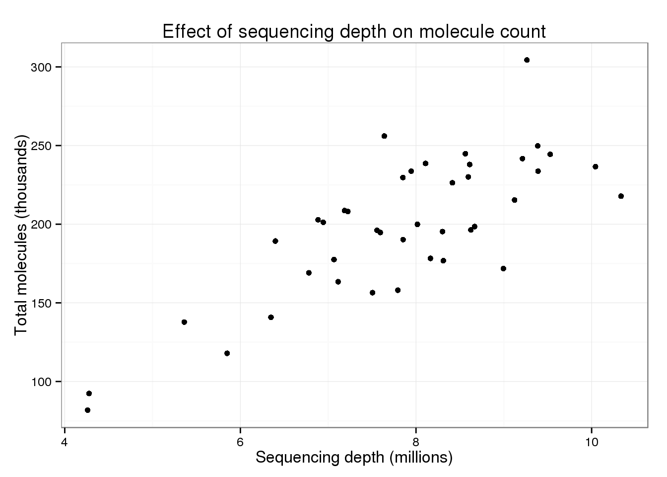

There is still a trend of more total molecules with increasing sequencing depth.

p_conv + geom_smooth(method = "lm")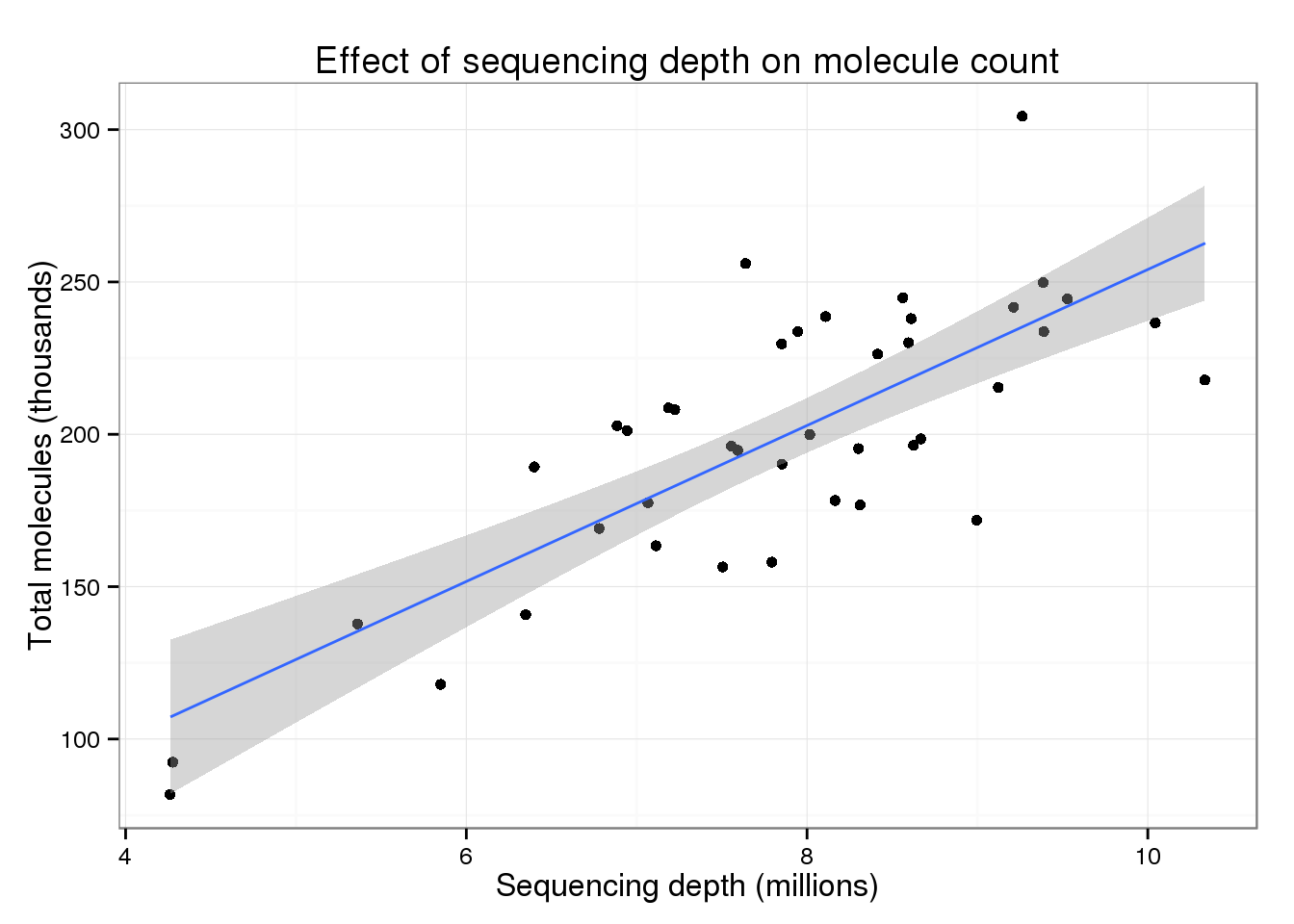

model_conv <- lm(total_molecules ~ total_reads, data = total_counts)
summary(model_conv)


Call:
lm(formula = total_molecules ~ total_reads, data = total_counts)

Residuals:
    Min      1Q  Median      3Q     Max 
-56.635 -19.889  -1.527  25.020  69.063 

Coefficients:
            Estimate Std. Error t value Pr(>|t|)    
(Intercept)   -1.896     26.053  -0.073    0.942    
total_reads   25.598      3.277   7.811  1.7e-09 ***
---
Signif. codes:  0 '***' 0.001 '**' 0.01 '*' 0.05 '.' 0.1 ' ' 1

Residual standard error: 28.3 on 39 degrees of freedom
Multiple R-squared:   0.61, Adjusted R-squared:    0.6 
F-statistic:    61 on 1 and 39 DF,  p-value: 1.698e-09

For every additional 1 million raw reads, a sample has ~25.6 thousand more molecules.

Session information

sessionInfo()

R version 3.2.0 (2015-04-16)
Platform: x86_64-unknown-linux-gnu (64-bit)

locale:
 [1] LC_CTYPE=en_US.UTF-8       LC_NUMERIC=C              
 [3] LC_TIME=en_US.UTF-8        LC_COLLATE=en_US.UTF-8    
 [5] LC_MONETARY=en_US.UTF-8    LC_MESSAGES=en_US.UTF-8   
 [7] LC_PAPER=en_US.UTF-8       LC_NAME=C                 
 [9] LC_ADDRESS=C               LC_TELEPHONE=C            
[11] LC_MEASUREMENT=en_US.UTF-8 LC_IDENTIFICATION=C       

attached base packages:
[1] stats     graphics  grDevices utils     datasets  methods   base     

other attached packages:
[1] ggplot2_1.0.1    data.table_1.9.4 BASiCS_0.3.0     knitr_1.10.5    

loaded via a namespace (and not attached):
 [1] Rcpp_0.12.0         magrittr_1.5        MASS_7.3-40        
 [4] BiocGenerics_0.14.0 munsell_0.4.2       colorspace_1.2-6   
 [7] lattice_0.20-31     stringr_1.0.0       httr_0.6.1         
[10] plyr_1.8.3          tools_3.2.0         parallel_3.2.0     
[13] grid_3.2.0          gtable_0.1.2        coda_0.17-1        
[16] htmltools_0.2.6     yaml_2.1.13         digest_0.6.8       
[19] reshape2_1.4.1      formatR_1.2         bitops_1.0-6       
[22] RCurl_1.95-4.6      evaluate_0.7        rmarkdown_0.6.1    
[25] labeling_0.3        stringi_0.4-1       scales_0.2.4       
[28] chron_2.3-45        proto_0.3-10

Islam et al (2014). Quantitative single-cell RNA-seq with unique molecular identifiers. Nature Methods 11: 163-166.↩