Correlations
John Blischak
2017-08-14
Last updated: 2018-01-29
Code version: f6b7f76
Calculate pairwise correlations between single cells.
Batch 1 only
Setup
library("cowplot")
library("dplyr")
library("edgeR")
library("ggplot2")
library("stringr")
library("tidyr")
theme_set(theme_cowplot())
library("Biobase") # has to be loaded last to use `combine`
Import data.
eset <- readRDS("../data/eset.rds")
eset
ExpressionSet (storageMode: lockedEnvironment)
assayData: 54792 features, 4992 samples
element names: exprs
protocolData: none
phenoData
sampleNames: 03162017-A01 03162017-A02 ... 12142017-H12 (4992
total)
varLabels: experiment well ... valid_id (40 total)
varMetadata: labelDescription
featureData
featureNames: ENSG00000000003 ENSG00000000005 ... WBGene00235374
(54792 total)
fvarLabels: chr start ... source (6 total)
fvarMetadata: labelDescription
experimentData: use 'experimentData(object)'
Annotation: Limit this analysis to batch 1 since it deals with the spike-ins.
eset <- eset[, eset$batch == "b1"]
dim(eset)
Features Samples
54792 960 Remove samples with bad cell number or TRA-1-60.
eset_quality <- eset[, eset$cell_number == 1 & eset$tra1.60]
dim(eset_quality)
Features Samples
54792 869 Separate by source.
eset_ce <- eset_quality[fData(eset_quality)$source == "C. elegans", ]
head(featureNames(eset_ce))
[1] "WBGene00000001" "WBGene00000002" "WBGene00000003" "WBGene00000004"
[5] "WBGene00000005" "WBGene00000006"eset_dm <- eset_quality[fData(eset_quality)$source == "D. melanogaster", ]
head(featureNames(eset_dm))[1] "FBgn0000008" "FBgn0000014" "FBgn0000015" "FBgn0000017" "FBgn0000018"
[6] "FBgn0000022"eset_ercc <- eset_quality[fData(eset_quality)$source == "ERCC",
eset_quality$ERCC != "Not added"]
head(featureNames(eset_ercc))[1] "ERCC-00002" "ERCC-00003" "ERCC-00004" "ERCC-00009" "ERCC-00012"
[6] "ERCC-00013"eset_hs <- eset_quality[fData(eset_quality)$source == "H. sapiens", ]
head(featureNames(eset_hs))[1] "ENSG00000000003" "ENSG00000000005" "ENSG00000000419" "ENSG00000000457"
[5] "ENSG00000000460" "ENSG00000000938"Define a function for filtering by percentage of cells in which a gene is detected.
present <- function(x, percent = 0.50) mean(x > 0) >= percentERCC
Remove zeros.
eset_ercc_clean <- eset_ercc[rowSums(exprs(eset_ercc)) != 0, ]
dim(eset_ercc_clean)
Features Samples
88 347 Only keep genes which are observed in at least 50% of the samples.
eset_ercc_clean <- eset_ercc_clean[apply(exprs(eset_ercc_clean), 1, present), ]
dim(eset_ercc_clean)
Features Samples
34 347 Convert to log2 counts per million.
mol_ercc_cpm <- cpm(exprs(eset_ercc_clean), log = TRUE)Calculate pairwise correlations.
cor_ercc <- cor(mol_ercc_cpm)
cor_ercc <- cor_ercc[upper.tri(cor_ercc)]
summary(cor_ercc)
Min. 1st Qu. Median Mean 3rd Qu. Max.
0.5247 0.8428 0.8861 0.8797 0.9261 0.9915 Drosophila
Remove zeros.
eset_dm_clean <- eset_dm[rowSums(exprs(eset_dm)) != 0, ]
dim(eset_dm_clean)
Features Samples
11561 869 Only keep genes which are observed in at least 50% of the samples.
eset_dm_clean <- eset_dm_clean[apply(exprs(eset_dm_clean), 1, present), ]
dim(eset_dm_clean)
Features Samples
327 869 Convert to log2 counts per million.
mol_dm_cpm <- cpm(exprs(eset_dm_clean), log = TRUE)Calculate pairwise correlations.
cor_dm <- cor(mol_dm_cpm)
cor_dm <- cor_dm[upper.tri(cor_dm)]
summary(cor_dm)
Min. 1st Qu. Median Mean 3rd Qu. Max.
-0.000496 0.319796 0.404290 0.410913 0.496175 0.791579 Drosophila - 5 pg
Select only samples that received 5 pg.
eset_dm_5pg <- eset_dm[, eset_dm$fly == 5000]
dim(eset_dm_5pg)
Features Samples
13832 343 Remove zeros.
eset_dm_5pg_clean <- eset_dm_5pg[rowSums(exprs(eset_dm_5pg)) != 0, ]
dim(eset_dm_5pg_clean)
Features Samples
9833 343 Only keep genes which are observed in at least 50% of the samples.
eset_dm_5pg_clean <- eset_dm_5pg_clean[apply(exprs(eset_dm_5pg_clean), 1, present), ]
dim(eset_dm_5pg_clean)
Features Samples
154 343 Convert to log2 counts per million.
mol_dm_5pg_cpm <- cpm(exprs(eset_dm_5pg_clean), log = TRUE)Calculate pairwise correlations.
cor_dm_5pg <- cor(mol_dm_5pg_cpm)
cor_dm_5pg <- cor_dm_5pg[upper.tri(cor_dm_5pg)]
summary(cor_dm_5pg)
Min. 1st Qu. Median Mean 3rd Qu. Max.
-0.1033 0.2268 0.2905 0.2912 0.3552 0.6254 Drosophila - 50 pg
Select only samples that received 50 pg.
eset_dm_50pg <- eset_dm[, eset_dm$fly == 50000]
dim(eset_dm_50pg)
Features Samples
13832 526 Remove zeros.
eset_dm_50pg_clean <- eset_dm_50pg[rowSums(exprs(eset_dm_50pg)) != 0, ]
dim(eset_dm_50pg_clean)
Features Samples
11120 526 Only keep genes which are observed in at least 50% of the samples.
eset_dm_50pg_clean <- eset_dm_50pg_clean[apply(exprs(eset_dm_50pg_clean), 1, present), ]
dim(eset_dm_50pg_clean)
Features Samples
530 526 Convert to log2 counts per million.
mol_dm_50pg_cpm <- cpm(exprs(eset_dm_50pg_clean), log = TRUE)Calculate pairwise correlations.
cor_dm_50pg <- cor(mol_dm_50pg_cpm)
cor_dm_50pg <- cor_dm_50pg[upper.tri(cor_dm_50pg)]
summary(cor_dm_50pg)
Min. 1st Qu. Median Mean 3rd Qu. Max.
0.2145 0.4689 0.5125 0.5108 0.5549 0.7243 C. elegans
Remove zeros.
eset_ce_clean <- eset_ce[rowSums(exprs(eset_ce)) != 0, ]
dim(eset_ce_clean)
Features Samples
13105 869 Only keep genes which are observed in at least 50% of the samples.
eset_ce_clean <- eset_ce_clean[apply(exprs(eset_ce_clean), 1, present), ]
dim(eset_ce_clean)
Features Samples
10 869 Convert to log2 counts per million.
mol_ce_cpm <- cpm(exprs(eset_ce_clean), log = TRUE)
# Remove samples with no observations for this subset
zeros_ce <- colSums(exprs(eset_ce_clean)) > 0
eset_ce_clean <- eset_ce_clean[, zeros_ce]
mol_ce_cpm <- mol_ce_cpm[, zeros_ce]
Calculate pairwise correlations.
cor_ce <- cor(mol_ce_cpm)
cor_ce <- cor_ce[upper.tri(cor_ce)]
summary(cor_ce)
Min. 1st Qu. Median Mean 3rd Qu. Max.
-0.2342 0.6687 0.7668 0.7449 0.8434 0.9997 Human
Remove zeros.
eset_hs_clean <- eset_hs[rowSums(exprs(eset_hs)) != 0, ]
dim(eset_hs_clean)
Features Samples
18904 869 Only keep genes which are observed in at least 50% of the samples.
eset_hs_clean <- eset_hs_clean[apply(exprs(eset_hs_clean), 1, present), ]
dim(eset_hs_clean)
Features Samples
6587 869 Convert to log2 counts per million.
mol_hs_cpm <- cpm(exprs(eset_hs_clean), log = TRUE)Calculate pairwise correlations.
cor_hs <- cor(mol_hs_cpm)
cor_hs <- cor_hs[upper.tri(cor_hs)]
summary(cor_hs)
Min. 1st Qu. Median Mean 3rd Qu. Max.
0.2404 0.4743 0.5472 0.5370 0.6003 0.7983 Summary plot
Below are the pairwise correlations for each source of RNA. The numbers along the bottom are the number of pairwise correlations included in each boxplot (not all samples received the same spike-ins).
boxplot(cor_ercc, cor_hs, cor_dm_50pg, cor_dm, cor_dm_5pg, cor_ce,
        names = c("ERCC", "Human", "Fly (50 pg)", "Fly (all)",
                  "Fly (5 pg)", "worm"),
        xlab = "Source", ylab = "Pearson correlation",
        main = "Pairwise correlations")
text(x = 1:6, y = -1, labels = sapply(list(cor_ercc, cor_hs, cor_dm_50pg, cor_dm, cor_dm_5pg, cor_ce), length))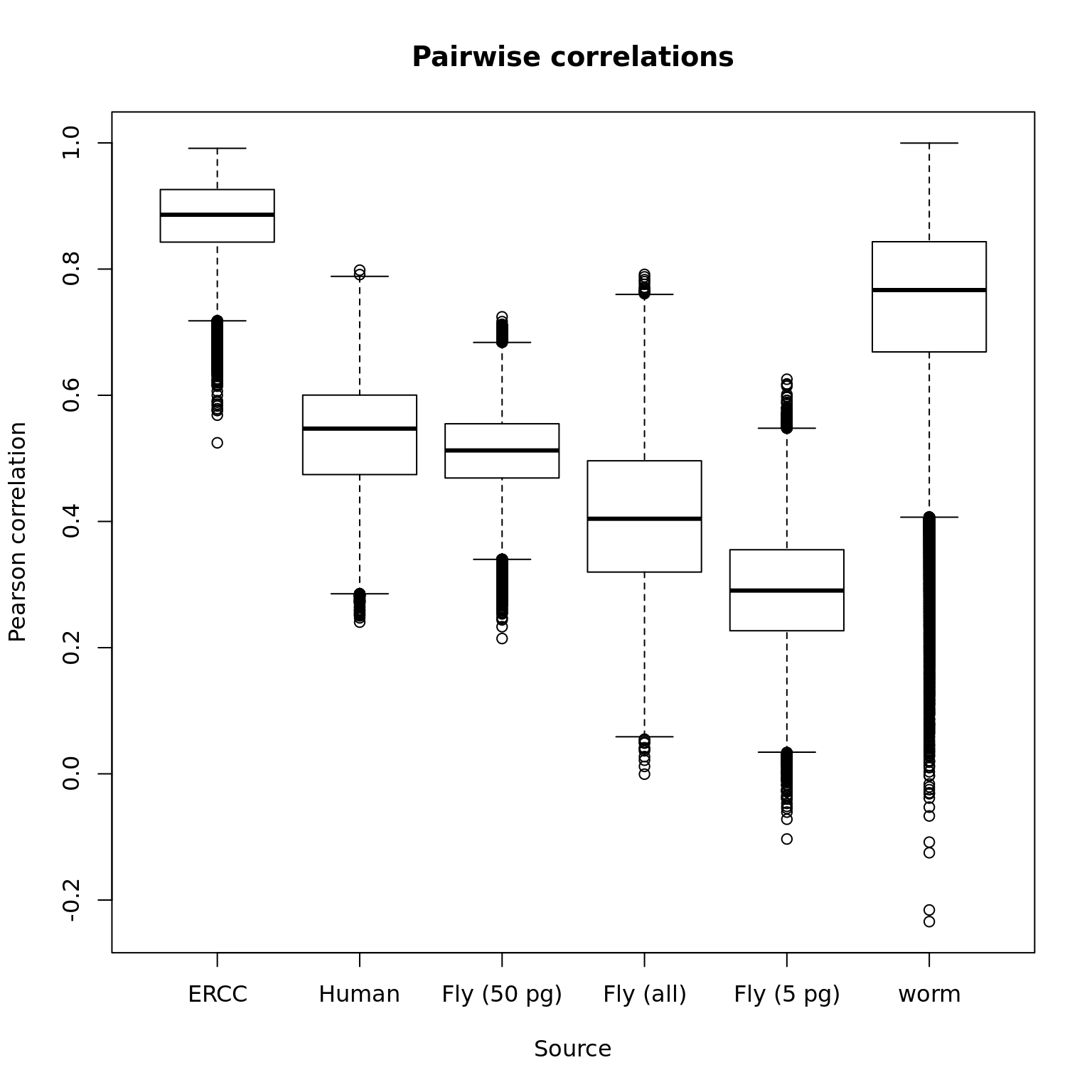
Pairwise correlations per C1 chip
Do the pairwise correlations change when looking within a chip versus between chips?
# Calculate pairwise correlations
#
# x - matrix produced by edger::cpm(). Column names should be of the form
# 03162017_A01
#
# id - optional character vector column
#
# method - a valid method to pass to cor()
calc_cor_pairs <- function(x, id = NULL, method = "pearson") {
  stopifnot(is.matrix(x),
            is.null(id) || (is.character(id) && length(id) == 1),
            method %in% c("pearson", "kendall", "spearman"))
  result <- x %>%
    cor(method = method) %>%
    as.data.frame %>%
    mutate(sample1 = colnames(x)) %>%
    gather(key = "sample2", value = "r", -sample1) %>%
    mutate(sample2 = as.character(sample2)) %>%
    filter(sample1 < sample2) %>% # only keep 1 of 2 duplicate entries
    arrange(sample1, sample2) %>%
    extract(col = sample1, into = c("experiment1", "well1"),
            regex = "([[:digit:]]+)-([[:alnum:]]+)") %>%
    extract(col = sample2, into = c("experiment2", "well2"),
            regex = "([[:digit:]]+)-([[:alnum:]]+)")
  n <- ncol(x)
  stopifnot(result$r < 1,
            nrow(result) == (n * n - n) / 2)
  if (!is.null(id)) {
    result$id <- id
  }
  return(result)
}
Cacluate pairwise correlations for each feature type and then combine them.
cor_long_dm <- calc_cor_pairs(mol_dm_cpm, id = "Fly")
cor_long_dm_5pg <- calc_cor_pairs(mol_dm_5pg_cpm, id = "Fly 5 pg")
cor_long_dm_50pg <- calc_cor_pairs(mol_dm_50pg_cpm, id = "Fly 50 pg")
cor_long_ercc <- calc_cor_pairs(mol_ercc_cpm, id = "ERCC")
cor_long_hs <- calc_cor_pairs(mol_hs_cpm, id = "Human")
cor_long <- rbind(cor_long_dm, cor_long_dm_5pg, cor_long_dm_50pg,
                  cor_long_ercc, cor_long_hs)
The pairwise correlations are only slightly higher within a chip versus between a chip.
cor_within_v_between <- cor_long %>%
  mutate(within = ifelse(experiment1 == experiment2,
                         "Within", "Between"))
ggplot(cor_within_v_between, aes(x = within, y = r)) +
  geom_boxplot() +
  facet_wrap(~id) +
  labs(title = "Pairwise correlations within versus between chips",
       x = "", y = "Correlation")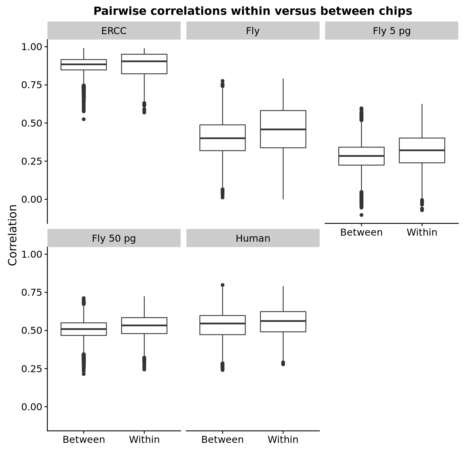
The pairwise correlations for a given RNA input source is similar across chips.
cor_per_chip <- cor_long %>%
  filter(experiment1 == experiment2)
ggplot(cor_per_chip, aes(x = id, y = r)) +
  geom_boxplot() +
  facet_wrap(~ experiment1) +
  labs(title = "Pairwise correlations per C1 chip",
       x = "", y = "Correlation") +
  theme(axis.text.x = element_text(angle = 45, hjust = 1, vjust = 1))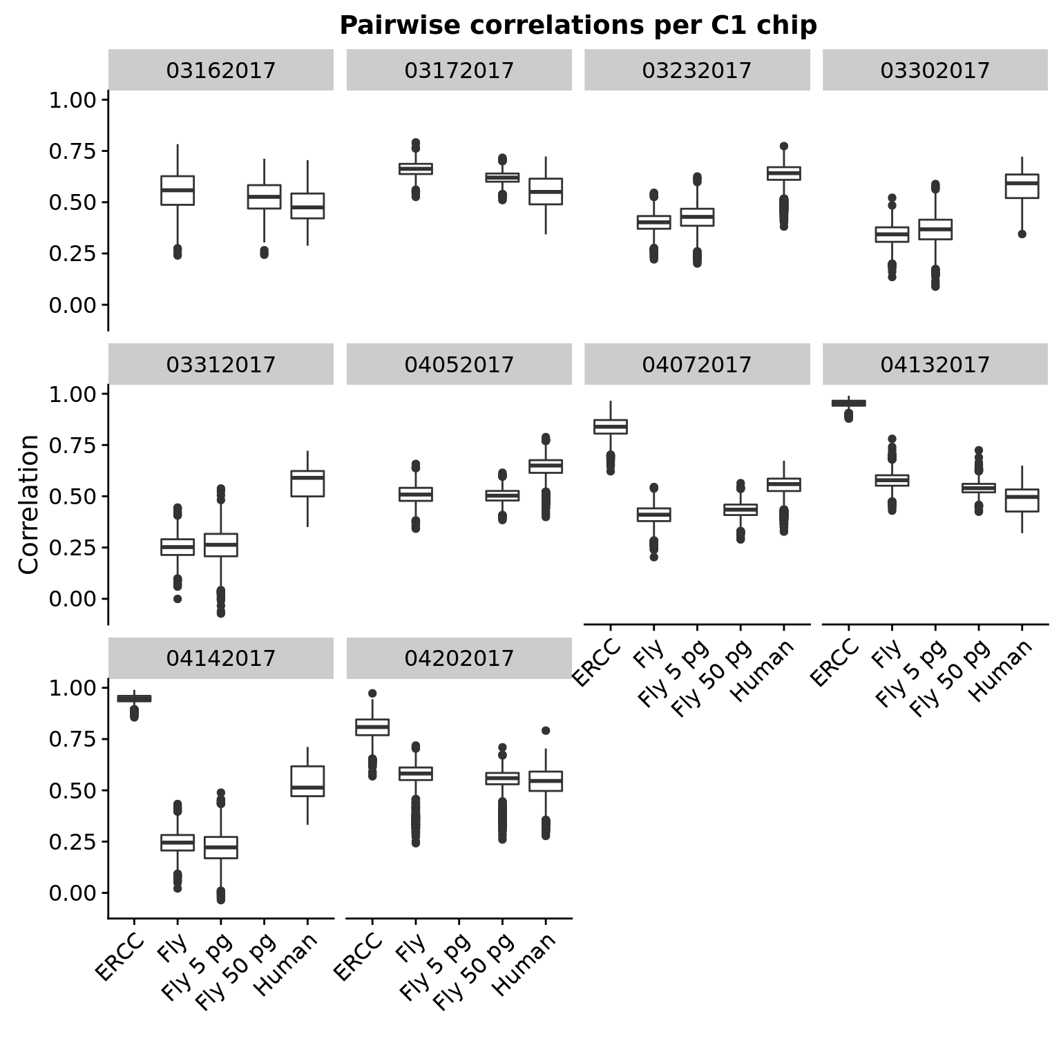
Note that the boxplots for Fly and Fly 5 or 50 pg are not identical even though each chip has only 1 because these were processed separately above when filtering genes which are present in at least 50% of samples.
Chip effect versus individual effect
anno <- pData(eset)
head(cor_long_hs)
experiment1 well1 experiment2 well2 r id
1 03162017 A01 03162017 A02 0.4527431 Human
2 03162017 A01 03162017 A03 0.3572271 Human
3 03162017 A01 03162017 A05 0.3968255 Human
4 03162017 A01 03162017 A06 0.4752021 Human
5 03162017 A01 03162017 A07 0.4369423 Human
6 03162017 A01 03162017 A08 0.4493643 Humancor_hs_long_cat <- cor_long_hs %>%
mutate(chip_id1 = anno[paste(experiment1, well1, sep = "-"), "chip_id"],
chip_id2 = anno[paste(experiment2, well2, sep = "-"), "chip_id"],
same_chip = experiment1 == experiment2,
same_ind = chip_id1 == chip_id2,
same_chip_same_ind = same_chip & same_ind,
same_chip_diff_ind = same_chip & !same_ind,
diff_chip_same_ind = !same_chip & same_ind,
diff_chip_diff_ind = !same_chip & !same_ind) %>%
gather("category", "assigned",
same_chip_same_ind:diff_chip_diff_ind) %>%
filter(assigned)The effect of individual is stronger than the effect of chip.
cor_hs_long_cat$category <- factor(cor_hs_long_cat$category,
                                   levels = c("same_chip_same_ind",
                                              "diff_chip_same_ind",
                                              "same_chip_diff_ind",
                                              "diff_chip_diff_ind"),
                                   labels = c("Same chip\nSame ind",
                                              "Diff chip\nSame ind",
                                              "Same chip\nDiff ind",
                                              "Diff chip\nDiff ind"))
ggplot(cor_hs_long_cat, aes(x = category, y = r)) +
  geom_boxplot() +
  labs(title = "Chip effect v. individual effect",
       x = "", y = "Pairwise Pearson correlations")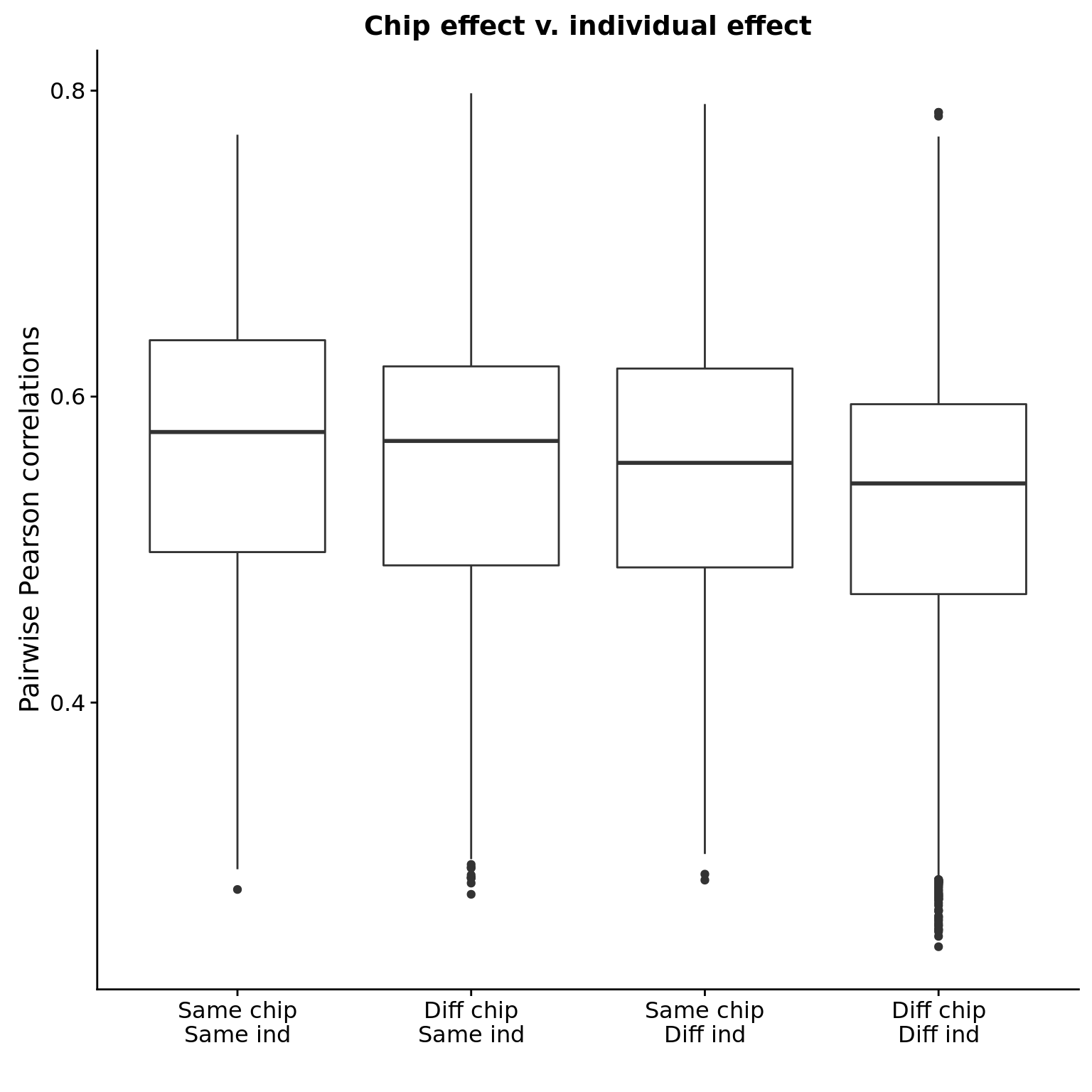
Session information
sessionInfo()R version 3.4.1 (2017-06-30)
Platform: x86_64-pc-linux-gnu (64-bit)
Running under: Scientific Linux 7.2 (Nitrogen)
Matrix products: default
BLAS: /project2/gilad/jdblischak/miniconda3/envs/scqtl/lib/R/lib/libRblas.so
LAPACK: /project2/gilad/jdblischak/miniconda3/envs/scqtl/lib/R/lib/libRlapack.so
locale:
[1] LC_CTYPE=en_US.UTF-8 LC_NUMERIC=C
[3] LC_TIME=en_US.UTF-8 LC_COLLATE=en_US.UTF-8
[5] LC_MONETARY=en_US.UTF-8 LC_MESSAGES=en_US.UTF-8
[7] LC_PAPER=en_US.UTF-8 LC_NAME=C
[9] LC_ADDRESS=C LC_TELEPHONE=C
[11] LC_MEASUREMENT=en_US.UTF-8 LC_IDENTIFICATION=C
attached base packages:
[1] parallel methods stats graphics grDevices utils datasets
[8] base
other attached packages:
[1] bindrcpp_0.2 Biobase_2.38.0 BiocGenerics_0.24.0
[4] tidyr_0.7.1 stringr_1.2.0 edgeR_3.20.1
[7] limma_3.34.1 dplyr_0.7.4 cowplot_0.9.1
[10] ggplot2_2.2.1
loaded via a namespace (and not attached):
[1] Rcpp_0.12.13 compiler_3.4.1 git2r_0.19.0 plyr_1.8.4
[5] bindr_0.1 tools_3.4.1 digest_0.6.12 evaluate_0.10.1
[9] tibble_1.3.3 gtable_0.2.0 lattice_0.20-34 pkgconfig_2.0.1
[13] rlang_0.1.2 yaml_2.1.14 knitr_1.16 tidyselect_0.2.3
[17] locfit_1.5-9.1 rprojroot_1.2 grid_3.4.1 glue_1.1.1
[21] R6_2.2.0 rmarkdown_1.6 purrr_0.2.2 magrittr_1.5
[25] backports_1.0.5 scales_0.5.0 htmltools_0.3.6 assertthat_0.1
[29] colorspace_1.3-2 labeling_0.3 stringi_1.1.2 lazyeval_0.2.0
[33] munsell_0.4.3 This R Markdown site was created with workflowr