Classifying musical genre using Spotify audio features
2024-05-22
Last updated: 2024-05-22
Checks: 7 0
Knit directory: stats352-spotify/
This reproducible R Markdown analysis was created with workflowr (version 1.7.1). The Checks tab describes the reproducibility checks that were applied when the results were created. The Past versions tab lists the development history.
Great! Since the R Markdown file has been committed to the Git repository, you know the exact version of the code that produced these results.
Great job! The global environment was empty. Objects defined in the global environment can affect the analysis in your R Markdown file in unknown ways. For reproduciblity it’s best to always run the code in an empty environment.
The command set.seed(20240522) was run prior to running
the code in the R Markdown file. Setting a seed ensures that any results
that rely on randomness, e.g. subsampling or permutations, are
reproducible.
Great job! Recording the operating system, R version, and package versions is critical for reproducibility.
Nice! There were no cached chunks for this analysis, so you can be confident that you successfully produced the results during this run.
Great job! Using relative paths to the files within your workflowr project makes it easier to run your code on other machines.
Great! You are using Git for version control. Tracking code development and connecting the code version to the results is critical for reproducibility.
The results in this page were generated with repository version 50e1f72. See the Past versions tab to see a history of the changes made to the R Markdown and HTML files.
Note that you need to be careful to ensure that all relevant files for
the analysis have been committed to Git prior to generating the results
(you can use wflow_publish or
wflow_git_commit). workflowr only checks the R Markdown
file, but you know if there are other scripts or data files that it
depends on. Below is the status of the Git repository when the results
were generated:
working directory clean
Note that any generated files, e.g. HTML, png, CSS, etc., are not included in this status report because it is ok for generated content to have uncommitted changes.
These are the previous versions of the repository in which changes were
made to the R Markdown (analysis/spotify.Rmd) and HTML
(docs/spotify.html) files. If you’ve configured a remote
Git repository (see ?wflow_git_remote), click on the
hyperlinks in the table below to view the files as they were in that
past version.
| File | Version | Author | Date | Message |
|---|---|---|---|---|
| Rmd | 50e1f72 | John Blischak | 2024-05-22 | wflow_publish("analysis/spotify.Rmd", delete_cache = TRUE) |
| html | 35c8864 | John Blischak | 2024-05-22 | Build site. |
| Rmd | e22daa6 | John Blischak | 2024-05-22 | Add spotify analysis |
This analysis attempts to classify songs into their correct musical genre using audio features. It is inspired by the original analysis by Kaylin Pavlik (@kaylinquest) in her 2019 blog post Understanding + classifying genres using Spotify audio features.
knitr::opts_chunk$set(autodep = TRUE)spotify <- read.csv("data/spotify.csv", stringsAsFactors = FALSE)
dim(spotify)[1] 32833 15head(spotify) genre danceability energy key loudness mode speechiness acousticness
1 pop 0.748 0.916 6 -2.634 1 0.0583 0.1020
2 pop 0.726 0.815 11 -4.969 1 0.0373 0.0724
3 pop 0.675 0.931 1 -3.432 0 0.0742 0.0794
4 pop 0.718 0.930 7 -3.778 1 0.1020 0.0287
5 pop 0.650 0.833 1 -4.672 1 0.0359 0.0803
6 pop 0.675 0.919 8 -5.385 1 0.1270 0.0799
instrumentalness liveness valence tempo duration_ms artist
1 0.00e+00 0.0653 0.518 122.036 194754 Ed Sheeran
2 4.21e-03 0.3570 0.693 99.972 162600 Maroon 5
3 2.33e-05 0.1100 0.613 124.008 176616 Zara Larsson
4 9.43e-06 0.2040 0.277 121.956 169093 The Chainsmokers
5 0.00e+00 0.0833 0.725 123.976 189052 Lewis Capaldi
6 0.00e+00 0.1430 0.585 124.982 163049 Ed Sheeran
song
1 I Don't Care (with Justin Bieber)
2 Memories
3 All the Time
4 Call You Mine
5 Someone You Loved
6 Beautiful People (feat. Khalid)table(spotify[, 1])
  edm latin   pop   r&b   rap  rock
 6043  5155  5507  5431  5746  4951
spotify <- spotify[, 1:13]Split the data into training and testing sets. The training set should have 3/4 of the samples.
numTrainingSamples <- nrow(spotify) * 3/4
trainingSet <- sample(seq_len(nrow(spotify)), size = numTrainingSamples)
spotifyTraining <- spotify[trainingSet, ]
spotifyTesting <- spotify[-trainingSet, ]
Build classification model with decision tree from the rpart package.
library("rpart")
model <- rpart(genre ~ ., data = spotifyTraining)
plot(model, margin = 0.05)
text(model)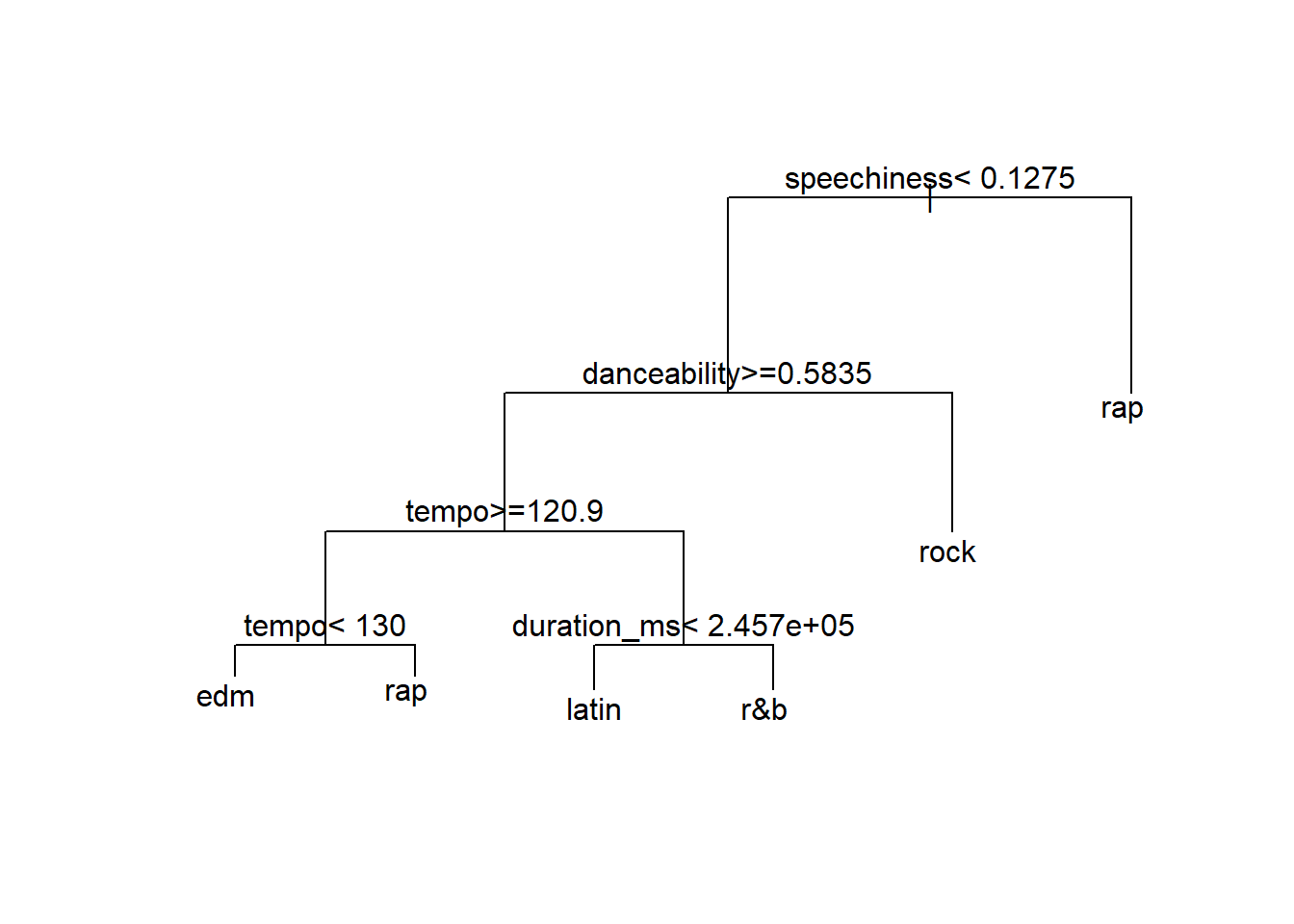
| Version | Author | Date |
|---|---|---|
| 35c8864 | John Blischak | 2024-05-22 |
Calculate prediction accuracy of the model on the training and testing sets.
predictTraining <- predict(model, type = "class")
(accuracyTraining <- mean(spotifyTraining[, 1] == predictTraining))
[1] 0.38763predictTesting <- predict(model, newdata = spotifyTesting[, -1], type = "class")
(accuracyTesting <- mean(spotifyTesting[, 1] == predictTesting))[1] 0.3821416Evaluate prediction performance using a confusion matrix.
table(predicted = predictTesting, observed = spotifyTesting[, 1]) observed
predicted edm latin pop r&b rap rock
edm 624 164 226 72 58 79
latin 162 494 404 261 155 133
pop 0 0 0 0 0 0
r&b 38 84 74 242 57 87
rap 337 470 316 540 1008 177
rock 360 105 377 233 103 769How does the model compare to random guessing?
predictRandom <- sample(unique(spotifyTesting[, 1]),
                        size = nrow(spotifyTesting),
                        replace = TRUE,
                        prob = table(spotifyTesting[, 1]))
(accuracyRandom <- mean(spotifyTesting[, 1] == predictRandom))
[1] 0.1525155
sessionInfo()R version 4.3.3 (2024-02-29 ucrt)
Platform: x86_64-w64-mingw32/x64 (64-bit)
Running under: Windows 11 x64 (build 22631)
Matrix products: default
locale:
[1] LC_COLLATE=English_United States.utf8
[2] LC_CTYPE=English_United States.utf8
[3] LC_MONETARY=English_United States.utf8
[4] LC_NUMERIC=C
[5] LC_TIME=English_United States.utf8
time zone: America/New_York
tzcode source: internal
attached base packages:
[1] stats graphics grDevices utils datasets methods base
other attached packages:
[1] rpart_4.1.23 workflowr_1.7.1
loaded via a namespace (and not attached):
[1] jsonlite_1.8.8 highr_0.10 compiler_4.3.3 promises_1.3.0
[5] Rcpp_1.0.12 stringr_1.5.1 git2r_0.33.0 callr_3.7.6
[9] later_1.3.2 jquerylib_0.1.4 yaml_2.3.8 fastmap_1.1.1
[13] R6_2.5.1 knitr_1.46 tibble_3.2.1 rprojroot_2.0.4
[17] bslib_0.7.0 pillar_1.9.0 rlang_1.1.3 utf8_1.2.4
[21] cachem_1.0.8 stringi_1.8.4 httpuv_1.6.15 xfun_0.43
[25] getPass_0.2-4 fs_1.6.4 sass_0.4.9 cli_3.6.2
[29] magrittr_2.0.3 ps_1.7.6 digest_0.6.35 processx_3.8.4
[33] rstudioapi_0.16.0 lifecycle_1.0.4 vctrs_0.6.5 evaluate_0.23
[37] glue_1.7.0 whisker_0.4.1 codetools_0.2-20 fansi_1.0.6
[41] rmarkdown_2.26 httr_1.4.7 tools_4.3.3 pkgconfig_2.0.3
[45] htmltools_0.5.8.1