2019-06-11-meteorites
John Blischak
2019-06-11
Last updated: 2019-06-11
Checks: 7 0
Knit directory: wflow-tidy-tuesday/
This reproducible R Markdown analysis was created with workflowr (version 1.4.0). The Checks tab describes the reproducibility checks that were applied when the results were created. The Past versions tab lists the development history.
Great! Since the R Markdown file has been committed to the Git repository, you know the exact version of the code that produced these results.
Great job! The global environment was empty. Objects defined in the global environment can affect the analysis in your R Markdown file in unknown ways. For reproduciblity it’s best to always run the code in an empty environment.
The command set.seed(20190611) was run prior to running the code in the R Markdown file. Setting a seed ensures that any results that rely on randomness, e.g. subsampling or permutations, are reproducible.
Great job! Recording the operating system, R version, and package versions is critical for reproducibility.
Nice! There were no cached chunks for this analysis, so you can be confident that you successfully produced the results during this run.
Great job! Using relative paths to the files within your workflowr project makes it easier to run your code on other machines.
Great! You are using Git for version control. Tracking code development and connecting the code version to the results is critical for reproducibility. The version displayed above was the version of the Git repository at the time these results were generated.
Note that you need to be careful to ensure that all relevant files for the analysis have been committed to Git prior to generating the results (you can use wflow_publish or wflow_git_commit). workflowr only checks the R Markdown file, but you know if there are other scripts or data files that it depends on. Below is the status of the Git repository when the results were generated:
Ignored files:
    Ignored:    .Rproj.user/
    Ignored:    docs/figure/
Note that any generated files, e.g. HTML, png, CSS, etc., are not included in this status report because it is ok for generated content to have uncommitted changes.
These are the previous versions of the R Markdown and HTML files. If you’ve configured a remote Git repository (see ?wflow_git_remote), click on the hyperlinks in the table below to view them.
| File | Version | Author | Date | Message |
|---|---|---|---|---|
| Rmd | b016af6 | John Blischak | 2019-06-11 | Add meteorites analysis. |
Introduction
Setup
library(lubridate)
library(tidyverse)
library(cowplot)
theme_set(theme_cowplot())
m <- read_csv("data/meteorites.csv")Exploration
head(m)# A tibble: 6 x 10
name id name_type class mass fall year lat long geolocation
<chr> <dbl> <chr> <chr> <dbl> <chr> <dbl> <dbl> <dbl> <chr>
1 Aachen 1 Valid L5 21 Fell 1880 50.8 6.08 (50.775, 6…
2 Aarhus 2 Valid H6 720 Fell 1951 56.2 10.2 (56.18333,…
3 Abee 6 Valid EH4 107000 Fell 1952 54.2 -113 (54.21667,…
4 Acapu… 10 Valid Acap… 1914 Fell 1976 16.9 -99.9 (16.88333,…
5 Achir… 370 Valid L6 780 Fell 1902 -33.2 -65.0 (-33.16667…
6 Adhi … 379 Valid EH4 4239 Fell 1919 32.1 71.8 (32.1, 71.…str(m)Classes 'spec_tbl_df', 'tbl_df', 'tbl' and 'data.frame': 45716 obs. of 10 variables:
$ name : chr "Aachen" "Aarhus" "Abee" "Acapulco" ...
$ id : num 1 2 6 10 370 379 390 392 398 417 ...
$ name_type : chr "Valid" "Valid" "Valid" "Valid" ...
$ class : chr "L5" "H6" "EH4" "Acapulcoite" ...
$ mass : num 21 720 107000 1914 780 ...
$ fall : chr "Fell" "Fell" "Fell" "Fell" ...
$ year : num 1880 1951 1952 1976 1902 ...
$ lat : num 50.8 56.2 54.2 16.9 -33.2 ...
$ long : num 6.08 10.23 -113 -99.9 -64.95 ...
$ geolocation: chr "(50.775, 6.08333)" "(56.18333, 10.23333)" "(54.21667, -113.0)" "(16.88333, -99.9)" ...
- attr(*, "spec")=
.. cols(
.. name = col_character(),
.. id = col_double(),
.. name_type = col_character(),
.. class = col_character(),
.. mass = col_double(),
.. fall = col_character(),
.. year = col_double(),
.. lat = col_double(),
.. long = col_double(),
.. geolocation = col_character()
.. )Expect name and id to be unique.
length(m$name) == length(unique(m$name))[1] TRUElength(m$id) == length(unique(m$id))[1] TRUE“Relict” meteorites are still assigned a class:
table(m$name_type, useNA = "ifany")
Relict  Valid
    75  45641
table(m$class[m$name_type == "Relict"])
Chondrite-fusion crust           Fusion crust               Relict H
                     4                      4                      1
           Relict iron              Relict OC
                     1                     65
There are lots of classes. Many are rare.
length(unique(m$class))[1] 455summary(as.numeric(table(m$class))) Min. 1st Qu. Median Mean 3rd Qu. Max.
1.0 1.0 4.0 100.5 17.0 8339.0 mass has some missing values, some zeros, and a strong right-skew.
summary(m$mass) Min. 1st Qu. Median Mean 3rd Qu. Max. NA's
0 7 33 13278 203 60000000 131 sum(m$mass == 0, na.rm = TRUE)[1] 19sum(m$mass > 10^5, na.rm = TRUE)[1] 282hist(log(m$mass))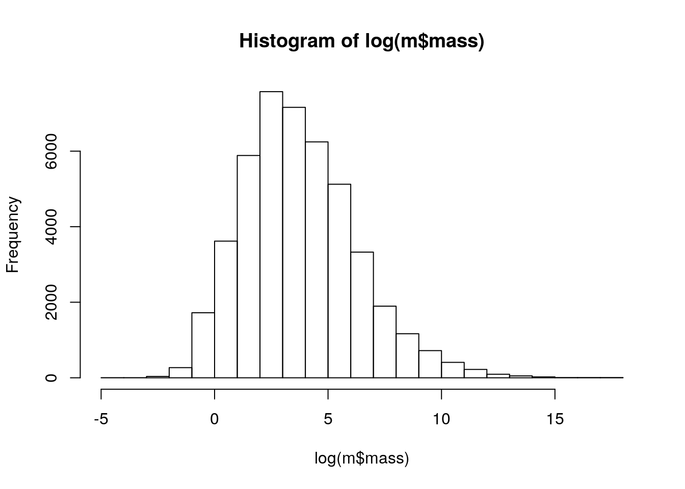
The meteorites are more often found rather than observed to fall (source).
table(m$fall, useNA = "ifany")
 Fell Found
 1107 44609
Most were found after 1900. One was found in the future.
summary(m$year) Min. 1st Qu. Median Mean 3rd Qu. Max. NA's
860 1987 1998 1992 2003 2101 291 hist(m$year)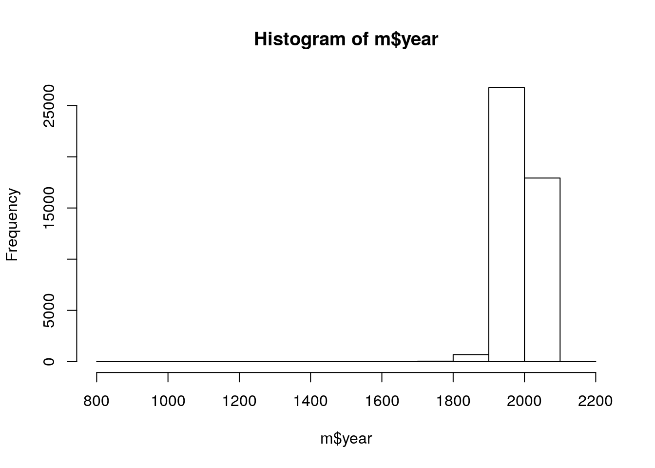
sum(m$year < 1900, na.rm = TRUE)[1] 728sum(m$year > year(now()), na.rm = TRUE)[1] 1Some meteorites are missing location data.
summary(m$lat) Min. 1st Qu. Median Mean 3rd Qu. Max. NA's
-87.37 -76.71 -71.50 -39.12 0.00 81.17 7315 summary(m$long) Min. 1st Qu. Median Mean 3rd Qu. Max. NA's
-165.43 0.00 35.67 61.07 157.17 354.47 7315 head(m$geolocation)[1] "(50.775, 6.08333)" "(56.18333, 10.23333)" "(54.21667, -113.0)"
[4] "(16.88333, -99.9)" "(-33.16667, -64.95)" "(32.1, 71.8)" sum(is.na(m$geolocation))[1] 7315sum(is.na(m$lat) & is.na(m$long) & is.na(m$geolocation))[1] 7315Clean
Remove difficult-to-classify meteorites and entries with missing values. Only keep meteorites found between 1900 and now.
m_clean <- m %>%
  na.omit %>%
  filter(name_type == "Valid",
         year <=  year(now()),
         year >= 1900) %>%
  select(name, class:geolocation)
nrow(m_clean)
[1] 37387head(m_clean)# A tibble: 6 x 8
name class mass fall year lat long geolocation
<chr> <chr> <dbl> <chr> <dbl> <dbl> <dbl> <chr>
1 Aarhus H6 720 Fell 1951 56.2 10.2 (56.18333, 10.2…
2 Abee EH4 107000 Fell 1952 54.2 -113 (54.21667, -113…
3 Acapulco Acapulco… 1914 Fell 1976 16.9 -99.9 (16.88333, -99.…
4 Achiras L6 780 Fell 1902 -33.2 -65.0 (-33.16667, -64…
5 Adhi Kot EH4 4239 Fell 1919 32.1 71.8 (32.1, 71.8)
6 Adzhi-Bogdo (… LL3-6 910 Fell 1949 44.8 95.2 (44.83333, 95.1…Questions
- What are the most common classes?
m_clean %>%
  group_by(class) %>%
  summarize(n = n()) %>%
  arrange(desc(n)) %>%
  filter(n > 1000)
# A tibble: 7 x 2
class n
<chr> <int>
1 L6 7457
2 H5 6193
3 H4 3869
4 H6 3852
5 L5 3255
6 LL5 2192
7 LL6 1649- Differences in fell versus found meteorites?
base_fall <- ggplot(m_clean, aes(x = fall)) + geom_boxplot()
base_fall %+% aes(y = year) + labs(title = "Difference in year")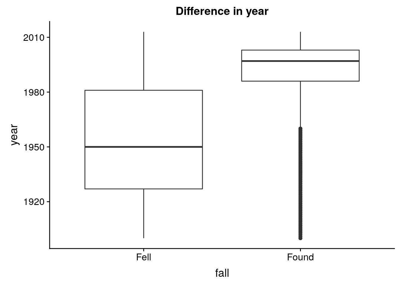
base_fall %+% aes(y = mass) + scale_y_log10() + labs(title = "Difference in size")Warning: Transformation introduced infinite values in continuous y-axisWarning: Removed 1 rows containing non-finite values (stat_boxplot).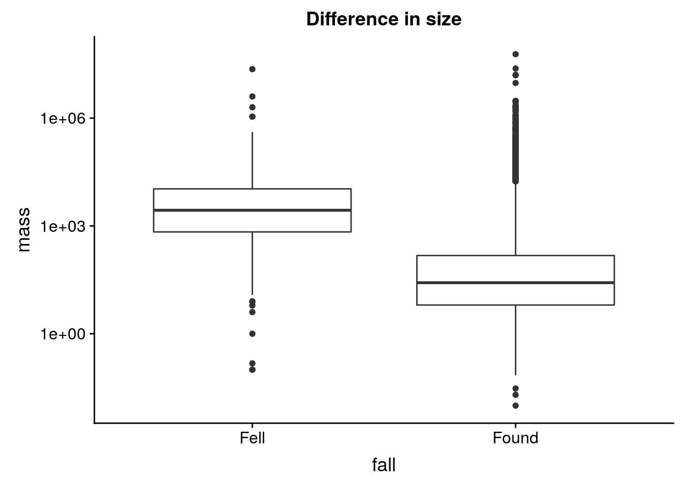
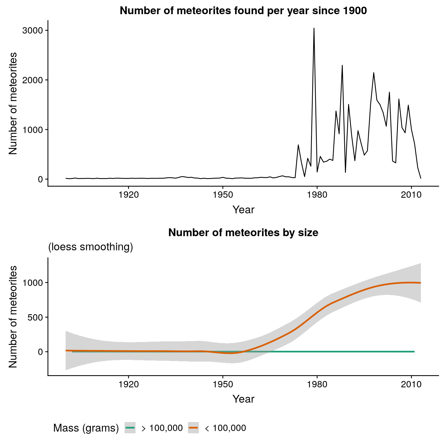
- Number and size of meteorites per year
m_per_year <- m_clean %>%
  group_by(year) %>%
  summarize(n = n(),
            mass_med = median(mass))
head(m_per_year)
# A tibble: 6 x 3
year n mass_med
<dbl> <int> <dbl>
1 1900 16 1350
2 1901 9 8400
3 1902 12 8510
4 1903 22 19140
5 1904 11 5700
6 1905 14 3132.ggplot(m_per_year, aes(x = year, y = n)) + geom_line() + geom_vline(xintercept = 1970, col = "red")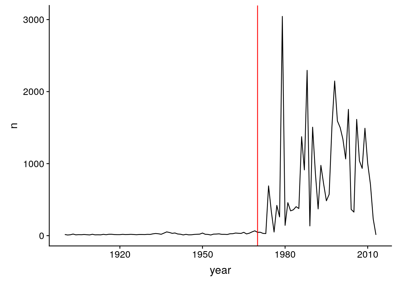
ggplot(m_per_year, aes(x = year, y = mass_med)) + geom_line() + geom_vline(xintercept = 1970, col = "red")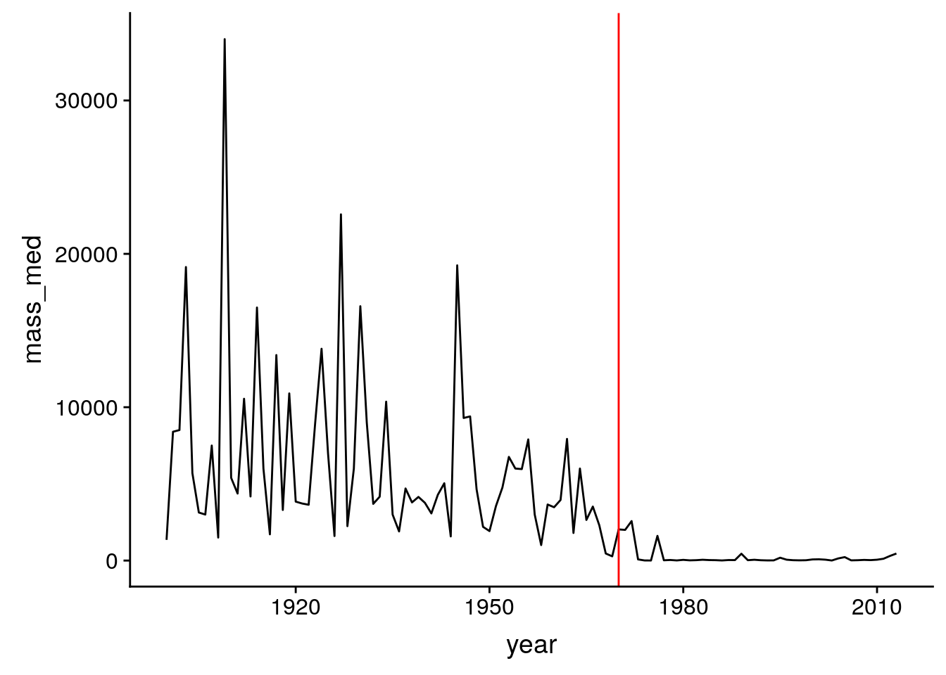
m_clean$size <- ifelse(m_clean$mass > 10^5, "big", "small")
m_per_year_size <- m_clean %>%
  group_by(year, size) %>%
  summarize(n = n(),
            mass_med = median(mass))
head(m_per_year_size)
# A tibble: 6 x 4
# Groups: year [4]
year size n mass_med
<dbl> <chr> <int> <dbl>
1 1900 small 16 1350
2 1901 small 9 8400
3 1902 big 1 15500000
4 1902 small 11 5720
5 1903 big 4 504500
6 1903 small 18 12150ggplot(m_per_year_size, aes(x = year, y = n, color = size)) + geom_smooth() + geom_vline(xintercept = 1970, col = "red")`geom_smooth()` using method = 'loess' and formula 'y ~ x'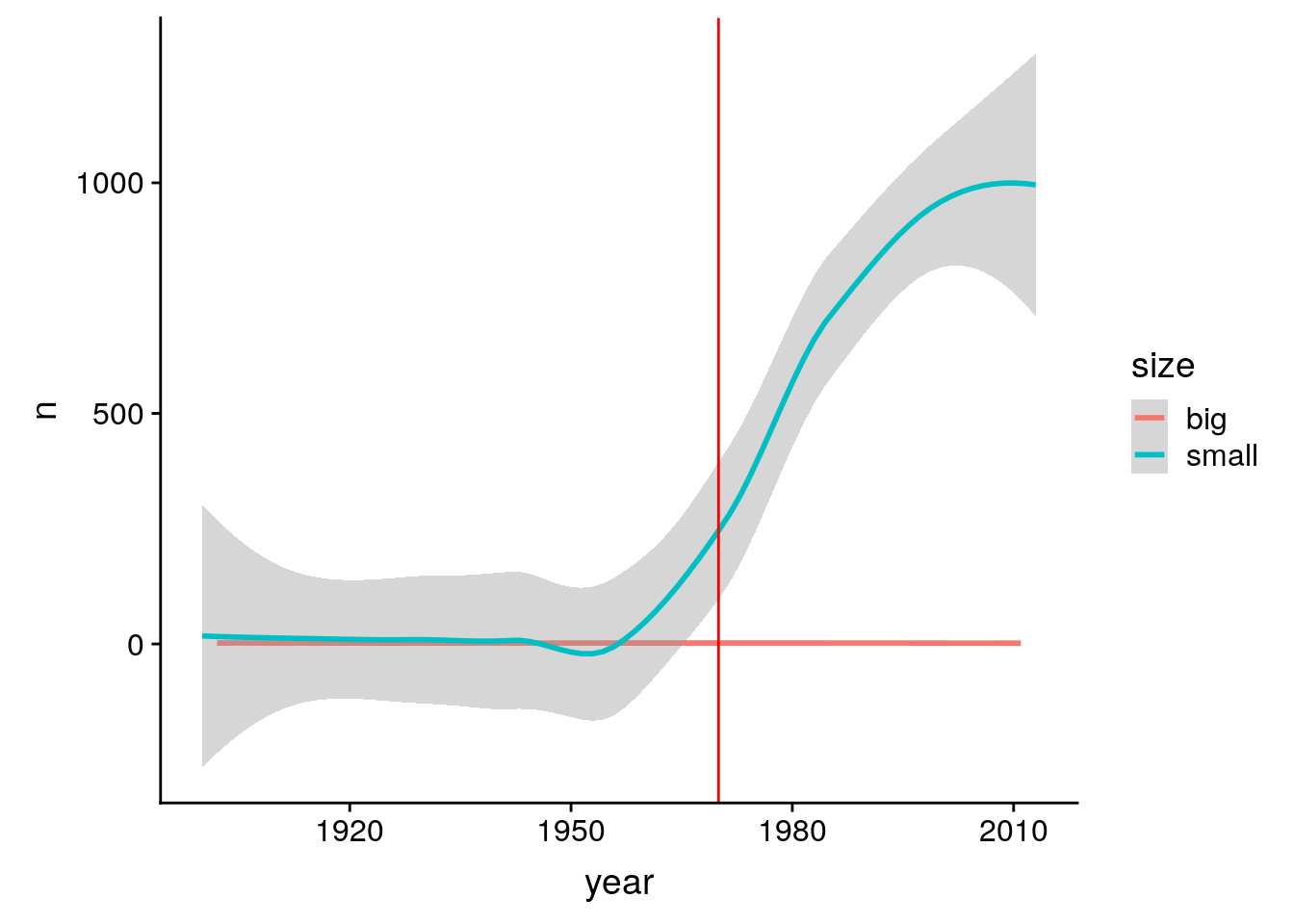
plot_grid(
  ggplot(m_per_year, aes(x = year, y = n)) +
    geom_line() +
    # geom_vline(xintercept = 1970, col = "red", linetype = "dashed") +
    labs(title = "Number of meteorites found per year since 1900",
         x = "Year", y = "Number of meteorites"),
  ggplot(m_per_year_size, aes(x = year, y = n, color = size)) +
    geom_smooth(method = "loess") +
    # geom_vline(xintercept = 1970, col = "red", linetype = "dashed") +
    labs(title = "Number of meteorites by size",
         x = "Year", y = "Number of meteorites",
         subtitle = "(loess smoothing)") +
    theme(legend.position = "bottom") +
    scale_color_brewer(name = "Mass (grams)",
                       labels = c("> 100,000", "< 100,000"), palette = "Dark2"),
  ncol = 1
)
sessionInfo()R version 3.6.0 (2019-04-26)
Platform: x86_64-pc-linux-gnu (64-bit)
Running under: Ubuntu 18.04.2 LTS
Matrix products: default
BLAS: /usr/lib/x86_64-linux-gnu/atlas/libblas.so.3.10.3
LAPACK: /usr/lib/x86_64-linux-gnu/atlas/liblapack.so.3.10.3
locale:
[1] LC_CTYPE=en_US.UTF-8 LC_NUMERIC=C
[3] LC_TIME=en_US.UTF-8 LC_COLLATE=en_US.UTF-8
[5] LC_MONETARY=en_US.UTF-8 LC_MESSAGES=en_US.UTF-8
[7] LC_PAPER=en_US.UTF-8 LC_NAME=C
[9] LC_ADDRESS=C LC_TELEPHONE=C
[11] LC_MEASUREMENT=en_US.UTF-8 LC_IDENTIFICATION=C
attached base packages:
[1] stats graphics grDevices utils datasets methods base
other attached packages:
[1] cowplot_0.9.4 forcats_0.4.0 stringr_1.4.0 dplyr_0.8.1
[5] purrr_0.3.2 readr_1.3.1 tidyr_0.8.3 tibble_2.1.3
[9] ggplot2_3.1.1 tidyverse_1.2.1 lubridate_1.7.4
loaded via a namespace (and not attached):
[1] tidyselect_0.2.5 xfun_0.7 haven_2.1.0
[4] lattice_0.20-38 vctrs_0.1.0 colorspace_1.4-1
[7] generics_0.0.2 htmltools_0.3.6 yaml_2.2.0
[10] utf8_1.1.4 rlang_0.3.4 pillar_1.4.1
[13] glue_1.3.1 withr_2.1.2 RColorBrewer_1.1-2
[16] modelr_0.1.4 readxl_1.3.1 plyr_1.8.4
[19] munsell_0.5.0 gtable_0.3.0 workflowr_1.4.0
[22] cellranger_1.1.0 rvest_0.3.4 evaluate_0.14
[25] labeling_0.3 knitr_1.23 fansi_0.4.0
[28] broom_0.5.2 Rcpp_1.0.1 scales_1.0.0
[31] backports_1.1.4 jsonlite_1.6 fs_1.3.1
[34] hms_0.4.2 digest_0.6.19 stringi_1.4.3
[37] grid_3.6.0 rprojroot_1.2 cli_1.1.0
[40] tools_3.6.0 magrittr_1.5 lazyeval_0.2.2
[43] zeallot_0.1.0 crayon_1.3.4 whisker_0.3-2
[46] pkgconfig_2.0.2 xml2_1.2.0 assertthat_0.2.1
[49] rmarkdown_1.13 httr_1.4.0 rstudioapi_0.10
[52] R6_2.4.0 nlme_3.1-140 git2r_0.25.2
[55] compiler_3.6.0