Cell-to-cell variation analysis: expressed cells
Joyce Hsiao
2016-07-01
- Background and some observations
- Set up
- Prepare data
- Compute gene mean and variance in the expressed cells
- CV-mean plots
- Extreme CV genes - top 1000
- Differential testing of adjusted CV - permutation
- Enrichment analysis of differential CV genes
- Supplemental tables for the manuscript
- Session information
Last updated: 2016-07-08
Code version: 641fc1222ff5c5bc6b4766ad24ea2f5420334427
Background and some observations
Compare expression variability among the detected/expressed cells between individuals. Our observations made in this document are summarized below.
CV-mean relationship: This pattern in the expressed cells is different from the usual concave function we observe in bulk RNA-seq and scRNA-seq. Gene CVs increase as a function of gene abundance for genes with more than 50 percent of undetected cells; while, gene CVs decrease as a function of mean abundance, a pattern similar to previous studies for genes with 50 percent or less undetected cells.
Overlaps of individual top mean and top CV genes: Similar to when including non-expressed cells, there are few common top CV genes across individuals (~100 genes) and many more common top genes across individuals ( > 800 genes). This suggests possible individual differences in expression variablity.
Compare CV of the expressed cells: We found 680 genes with differential variation across the expressed cell.
Compare mean abundance of the expressed cells: Due to the large number of cells in each individual cell lines, more than 95% of the genes were found to have statistically significant differences between all three individuals. We identified differential expression genes between pairs of individuals under the conditions of q-value less than .01 in the test and also log2 fold change greater than 2: 5 genes in NA19098-NA19101, 6 in NA19098-NA19239, and 2 genes in NA19101-NA19239. Note: The criterion for differential expression genes may be stringent, but the goal of this analysis is not to have a final say on the biological differences between the cell line, but rather to begin a conversatoin about the relationship between percent of undeteced cells and mean abundance
Set up
library(knitr)
library("ggplot2")
library("grid")
theme_set(theme_bw(base_size = 12))
source("functions.R")
library("Humanzee")
library("cowplot")
library("MASS")
library("matrixStats")
source("../code/cv-functions.r")
source("../code/plotting-functions.R")
library("mygene")
Prepare data
We import molecule counts before standardizing and transformation and also log2-transformed counts after batch-correction. Biological variation analysis of the individuals is performed on the batch-corrected and log2-transformed counts.
# Import filtered annotations
anno_filter <- read.table("../data/annotation-filter.txt",
                      header = TRUE,
                      stringsAsFactors = FALSE)

# Import filtered molecule counts
molecules_filter <- read.table("../data/molecules-filter.txt",
                               header = TRUE, stringsAsFactors = FALSE)
stopifnot(NROW(anno_filter) == NCOL(molecules_filter))

# Import final processed molecule counts of endogeneous genes
molecules_final <- read.table("../data/molecules-final.txt",
                             header = TRUE, stringsAsFactors = FALSE)
stopifnot(NROW(anno_filter) == NCOL(molecules_final))

# Import gene symbols
gene_symbols <- read.table(file = "../data/gene-info.txt", sep = "\t",
                           header = TRUE, stringsAsFactors = FALSE, quote = "")

# Import cell-cycle gene list
cell_cycle_genes <- read.table("../data/cellcyclegenes.txt",
                               header = TRUE, sep = "\t",
                               stringsAsFactors = FALSE)

# Import pluripotency gene list
pluripotency_genes <- read.table("../data/pluripotency-genes.txt",
                               header = TRUE, sep = "\t",
                               stringsAsFactors = FALSE)$To
Load CV results of all cells from previous analysis
load("../data/cv-all-cells.rda")Compute gene mean and variance in the expressed cells
file_name <- "../data/cv-expressed-cells.rda"
if (file.exists(file_name)) {
  load(file_name)
} else {
expressed_cv <- compute_expressed_cv(molecules_filter,
                                     molecules_final,
                                     anno_filter$individual)

expressed_dm <- normalize_cv_input(expressed_cv,
                                   anno_filter$individual)

save(expressed_cv, expressed_dm, file = file_name)
}
str(expressed_cv)
List of 4
$ NA19098:'data.frame': 13043 obs. of 3 variables:
..$ expr_mean: num [1:13043] 108.7 244.2 93.2 212.7 295.3 ...
..$ expr_var : num [1:13043] 2374 16242 1785 13192 18436 ...
..$ expr_cv : num [1:13043] 0.448 0.522 0.453 0.54 0.46 ...
$ NA19101:'data.frame': 13043 obs. of 3 variables:
..$ expr_mean: num [1:13043] 187 342 160 277 504 ...
..$ expr_var : num [1:13043] 7904 40164 3376 24609 81237 ...
..$ expr_cv : num [1:13043] 0.475 0.586 0.362 0.567 0.565 ...
$ NA19239:'data.frame': 13043 obs. of 3 variables:
..$ expr_mean: num [1:13043] 147 352 154 313 337 ...
..$ expr_var : num [1:13043] 2257 38260 2594 41557 32277 ...
..$ expr_cv : num [1:13043] 0.323 0.556 0.331 0.651 0.533 ...
$ all :'data.frame': 13043 obs. of 3 variables:
..$ expr_mean: num [1:13043] 154 321 143 274 386 ...
..$ expr_var : num [1:13043] 5575 35137 3377 30136 54273 ...
..$ expr_cv : num [1:13043] 0.484 0.585 0.407 0.634 0.603 ...13,043 genes were found to have valid CV and normalized CV (dm) measures in our computations that use a subset of cells with more than 1 UMI. This set of genes is smaller than the 13,058 genes in the final dataset (molecules-final.txt). The difference of 15 genes is the result of filtering out genes that do not have valid CV measures in all of the individuals; these are also genes that we did not detect a UMI in at least one of the individuals.
diff_set <- setdiff(as.character(rownames(molecules_final)),
                    as.character(rownames(expressed_cv$all)) )
for (i in 1:length(diff_set)) {
print(
  table(unlist(molecules_filter[rownames(molecules_filter) == diff_set[i], ]) > 1, anno_filter$individual) )
}
        NA19098 NA19101 NA19239
  FALSE     142     200     212
  TRUE        0       1       9

        NA19098 NA19101 NA19239
  FALSE     142     200     208
  TRUE        0       1      13

        NA19098 NA19101 NA19239
  FALSE     142     201     221

        NA19098 NA19101 NA19239
  FALSE     142     200     168
  TRUE        0       1      53

        NA19098 NA19101 NA19239
  FALSE     142     174     147
  TRUE        0      27      74

        NA19098 NA19101 NA19239
  FALSE     138     201     221
  TRUE        4       0       0

        NA19098 NA19101 NA19239
  FALSE     142     186     221
  TRUE        0      15       0

        NA19098 NA19101 NA19239
  FALSE     103     181     221
  TRUE       39      20       0

        NA19098 NA19101 NA19239
  FALSE     142     193     221
  TRUE        0       8       0

        NA19098 NA19101 NA19239
  FALSE     142     178     201
  TRUE        0      23      20

        NA19098 NA19101 NA19239
  FALSE     126     193     221
  TRUE       16       8       0

        NA19098 NA19101 NA19239
  FALSE     142     197     211
  TRUE        0       4      10

        NA19098 NA19101 NA19239
  FALSE     142     201     215
  TRUE        0       0       6

        NA19098 NA19101 NA19239
  FALSE       0       2     221
  TRUE      142     199       0

        NA19098 NA19101 NA19239
  FALSE     142     191     219
  TRUE        0      10       2
We subset the expression matrices of the 13,058 genes to include only the 13,043 genes with valid CV measures.
# get gene names from the cv data of the expessed cells
valid_genes_cv_expressed <- rownames(expressed_cv[[1]])

# make subset data for later analysis involving expressed cells
molecules_filter_subset <- molecules_filter[
  which(rownames(molecules_filter) %in% valid_genes_cv_expressed), ]

molecules_final_subset <- molecules_final[
  which(rownames(molecules_final) %in% valid_genes_cv_expressed), ]

# subset cv for all cells to include only the 13,043 genes with valid measures of CV among the expressed cells
ENSG_cv_subset <- lapply(ENSG_cv, function(x) {
  x[which(rownames(x) %in% valid_genes_cv_expressed), ]
})
names(ENSG_cv_subset) <- names(ENSG_cv)

# subset adjusted cv for all cells to include only the 13,043 genes with valid measures of CV among the expressed cells
ENSG_cv_adj_subset <- lapply(ENSG_cv_adj, function(x) {
  x[which(rownames(x) %in% valid_genes_cv_expressed), ]
})
names(ENSG_cv_adj_subset) <- names(ENSG_cv_adj)
Compute a matrix of 0’s and 1’s indicating non-detected and detected cells, respectively.
molecules_expressed_subset <- molecules_filter_subset
molecules_expressed_subset[which(molecules_filter_subset > 0 , arr.ind = TRUE)] <- 1
molecules_expressed_subset <- as.matrix((molecules_expressed_subset))

# make a batch-corrected data set in which the non-detected cells are
# code as NA
molecules_final_expressed_subset <- molecules_final_subset
molecules_final_expressed_subset[which(molecules_filter_subset == 0, arr.ind= TRUE)] <- NA
CV-mean plots
theme_set(theme_bw(base_size = 8))
cowplot::plot_grid(
    plot_poisson_cv_expressed(
          expr_mean = expressed_cv$all$expr_mean,
          exprs_cv = expressed_cv$all$expr_cv,
          ylab = "Coefficient of variation (CV)",
          main = "All individauls, expressed cells") +
          theme(legend.position = "none"),
    plot_poisson_cv_expressed(
          expr_mean = expressed_cv$NA19098$expr_mean,
          exprs_cv = expressed_cv$NA19098$expr_cv,
          ylab = "Coefficient of variation (CV)",
          main = "NA19098 expressed cells") +
          theme(legend.position = "none"),
    plot_poisson_cv_expressed(
          expr_mean = expressed_cv$NA19101$expr_mean,
          exprs_cv = expressed_cv$NA19101$expr_cv,
          ylab = "Coefficient of variation (CV)",
          main = "NA19101 expressed cells") +
          theme(legend.position = "none"),
    plot_poisson_cv_expressed(
          expr_mean = expressed_cv$NA19239$expr_mean,
          exprs_cv = expressed_cv$NA19239$expr_cv,
          ylab = "Coefficient of variation (CV)",
          main = "NA19239 expressed cells") +
          theme(legend.position = "none"),
  ncol = 2,
  labels = LETTERS[1:4])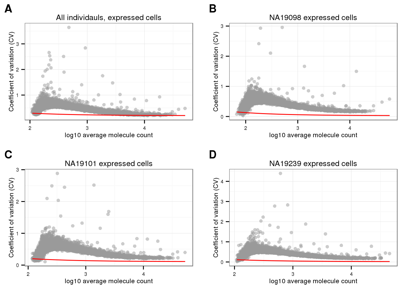
CV all cells vs. expressed cells
require(matrixStats)

xlabs <- "CV of all cells"
ylabs <- "CV of expressed cells"
plot_title <- names(expressed_cv)
par(mfrow = c(2,2))
# plot(x = ENSG_cv_subset$all$cv,
#      y = expressed_cv$all$expr_cv)
for (ind in names(expressed_cv)[1:3]) {
  which_ind <- which(names(ENSG_cv_subset) %in% ind)
  plot(x = ENSG_cv_subset[[ind]]$cv,
       y = expressed_cv[[ind]]$expr_cv,
       cex = .7, pch = 16, col = scales::alpha("grey20", .7),
       xlab = xlabs,
       ylab = ylabs,
       main = plot_title[which_ind])
}
title("CV before adjustment")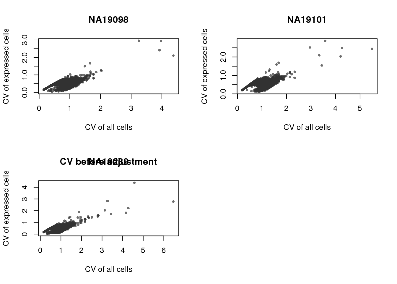
Adjusted CV values are orthogonal between individuals.
par(mfrow = c(2,2))
for (i in 1:2) {
  for (j in (i+1):3) {
    plot(expressed_cv[[i]]$expr_cv,
         expressed_cv[[j]]$expr_cv,
         xlab = names(expressed_cv)[i],
         ylab = names(expressed_cv)[j],
          cex = .7, pch = 16, col = scales::alpha("grey20", .7))
  }
}
title(main = "Between individual CVs",
      outer = TRUE, line = -1)


par(mfrow = c(2,2))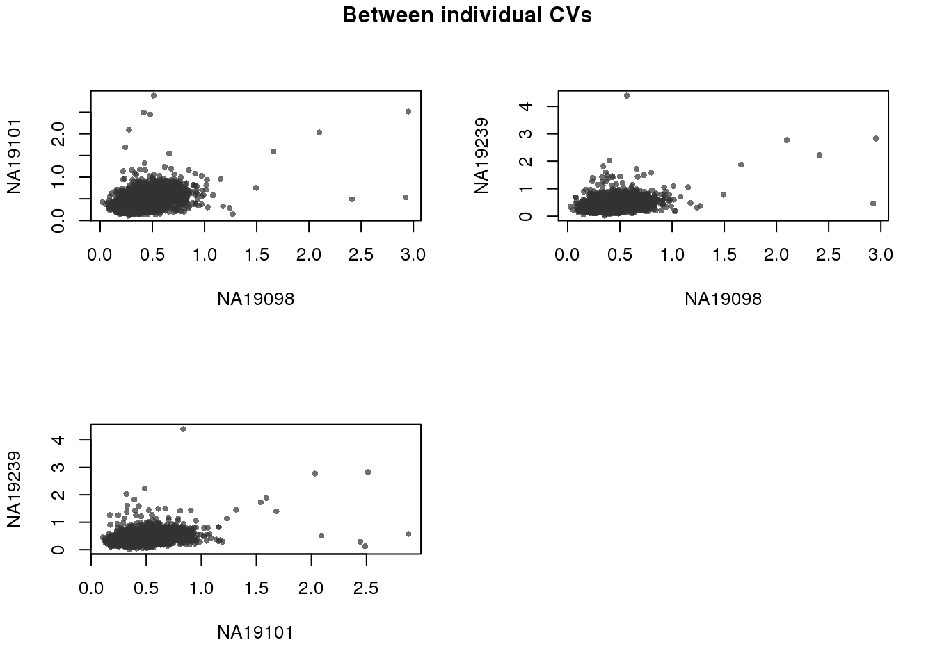
for (i in 1:2) {
  for (j in (i+1):3) {
    plot(expressed_dm[[i]],
         expressed_dm[[j]],
         xlab = names(expressed_cv)[i],
         ylab = names(expressed_cv)[j],
          cex = .7, pch = 16, col = scales::alpha("grey20", .7))
  }
}
title(main = "Between individual adjusted CVs",
      outer = TRUE, line = -1)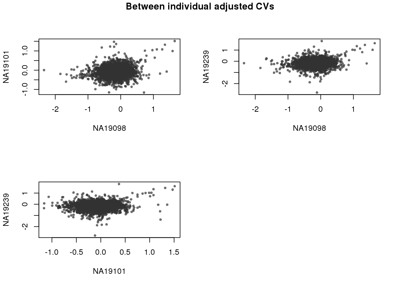
Extreme CV genes - top 1000
CV before correction
library(VennDiagram)
library(gridExtra)
genes <- rownames(molecules_final_subset)
overlap_list_expressed <- list(
   NA19098 = genes[ which( rank(expressed_cv$NA19098$expr_cv)
                               > length(genes) - 1000 ) ],
   NA19101 = genes[ which( rank(expressed_cv$NA19101$expr_cv)
                               > length(genes) - 1000 ) ],
   NA19239 = genes[ which( rank(expressed_cv$NA19239$expr_cv)
                               > length(genes) - 1000 ) ] )

overlap_list_all <- list(
   NA19098 = genes[ which( rank(ENSG_cv_subset$NA19098$cv)
                               > length(genes) - 1000 ) ],
   NA19101 = genes[ which( rank(ENSG_cv_subset$NA19101$cv)
                           > length(genes) - 1000 ) ],
   NA19239 = genes[ which( rank(ENSG_cv_subset$NA19239$cv)
                           > length(genes) - 1000 ) ] )

grid.arrange(gTree(children = venn.diagram(overlap_list_all,filename = NULL,
                          category.names = names(overlap_list_all),
                          name = "All cells")),
             gTree(children = venn.diagram(overlap_list_expressed,filename = NULL,
                          category.names = names(overlap_list_expressed),
                          name = "Expressed cells")),
             ncol = 2)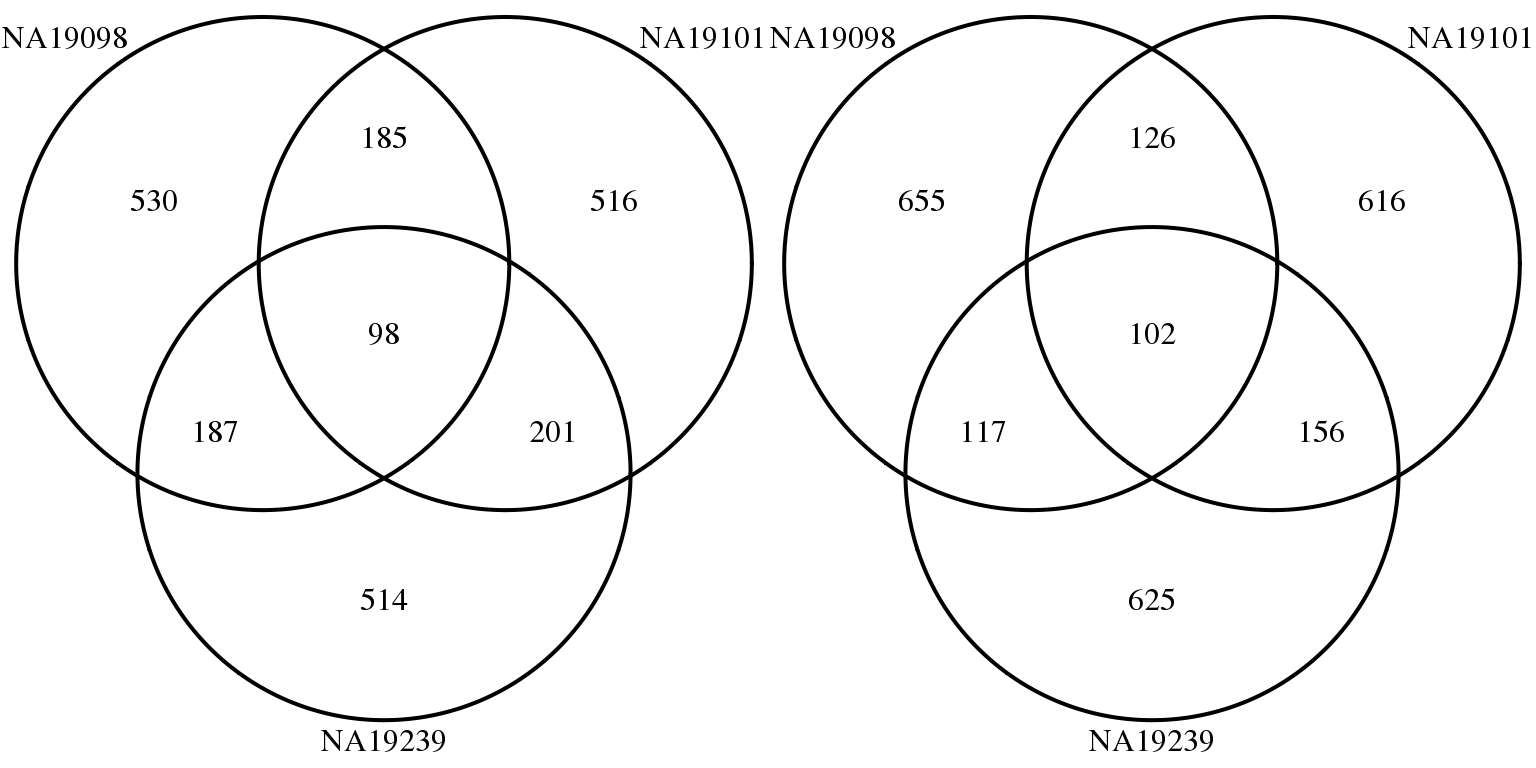
Adjusted CV (CV after correction for mean abundance)
genes <- rownames(molecules_final_subset)
overlap_list_expressed <- list(
   NA19098 = genes[ which( rank(expressed_dm$NA19098)
                               > length(genes) - 1000 ) ],
   NA19101 = genes[ which( rank(expressed_dm$NA19101)
                               > length(genes) - 1000 ) ],
   NA19239 = genes[ which( rank(expressed_dm$NA19239)
                               > length(genes) - 1000 ) ] )

overlap_list_all <- list(
   NA19098 = genes[ which( rank(ENSG_cv_adj_subset$NA19098$log10cv2_adj)
                               > length(genes) - 1000 ) ],
   NA19101 = genes[ which( rank(ENSG_cv_adj_subset$NA19101$log10cv2_adj)
                           > length(genes) - 1000 ) ],
   NA19239 = genes[ which( rank(ENSG_cv_adj_subset$NA19239$log10cv2_adj)
                           > length(genes) - 1000 ) ] )

grid.arrange(gTree(children = venn.diagram(overlap_list_all,filename = NULL,
                          category.names = names(overlap_list_all),
                          name = "All cells")),
             gTree(children = venn.diagram(overlap_list_expressed,filename = NULL,
                          category.names = names(overlap_list_expressed),
                          name = "Expressed cells")),
             ncol = 2)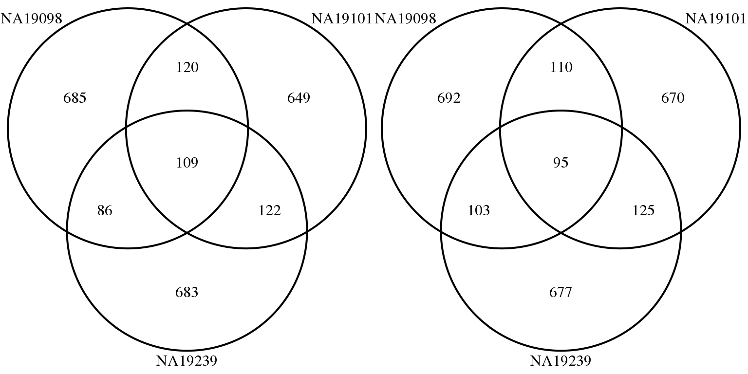
Mean and CV
genes <- rownames(molecules_final_subset)
overlap_list_expressed <- list(
   NA19098 = genes[ which( rank(expressed_dm$NA19098)
                               > length(genes) - 1000 ) ],
   NA19101 = genes[ which( rank(expressed_dm$NA19101)
                               > length(genes) - 1000 ) ],
   NA19239 = genes[ which( rank(expressed_dm$NA19239)
                               > length(genes) - 1000 ) ] )

overlap_list_mn <- list(
   NA19098 = genes[ which( rank(expressed_cv$NA19098$expr_mean)
                               > length(genes) - 1000 ) ],
   NA19101 = genes[ which( rank(expressed_cv$NA19101$expr_mean)
                           > length(genes) - 1000 ) ],
   NA19239 = genes[ which( rank(expressed_cv$NA19239$expr_mean)
                           > length(genes) - 1000 ) ] )

grid.arrange(gTree(children = venn.diagram(overlap_list_expressed,filename = NULL,
                          category.names = names(overlap_list_expressed),
                          name = "Adjusted CV")),
             gTree(children = venn.diagram(overlap_list_mn,filename = NULL,
                          category.names = names(overlap_list_mn),
                          name = "Abundance")),
             ncol = 2)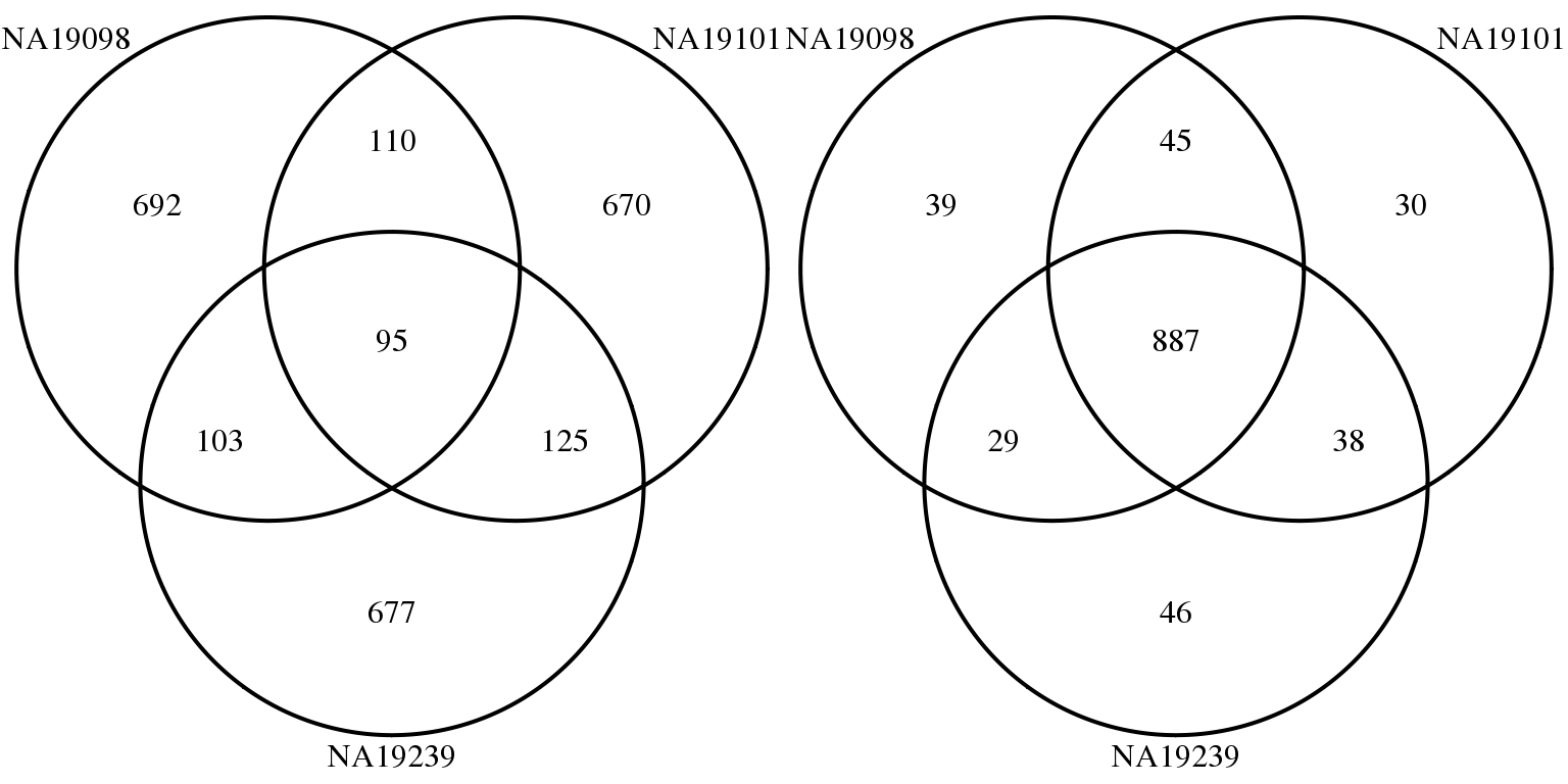
Differential testing of adjusted CV - permutation
Compute MAD values.
library(matrixStats)
mad_expressed <- rowMedians( abs( as.matrix(expressed_dm) - rowMedians(as.matrix(expressed_dm)) ) )
#save(mad_expressed, file = "../data/mad-expressed.rda")
Load empirical p-values of the MAD values. The permutations were done in midway.
Method: After obtaining the number of permutated statistics greatert than each observed test statistic, we follow the method by Philson and Smyth (2010) and compute the emprical p-value as \(p = (b+1)/(m+1)\) where \(b\) is the number of the permutation-based test statistics that are more significant than the observed test statistics, and \(m\) is the number of permutations performed.
permuted-pval-expressed-set1.rda: 300,000 permutations
load("../data/permuted-pval-expressed-set1.rda")
load("../data/mad-expressed.rda")
par(mfrow = c(1,1))
hist(perm_pval_set1,
     main = paste(m_perm_set1, "permutations"),
     xlab = "Empirical p-value")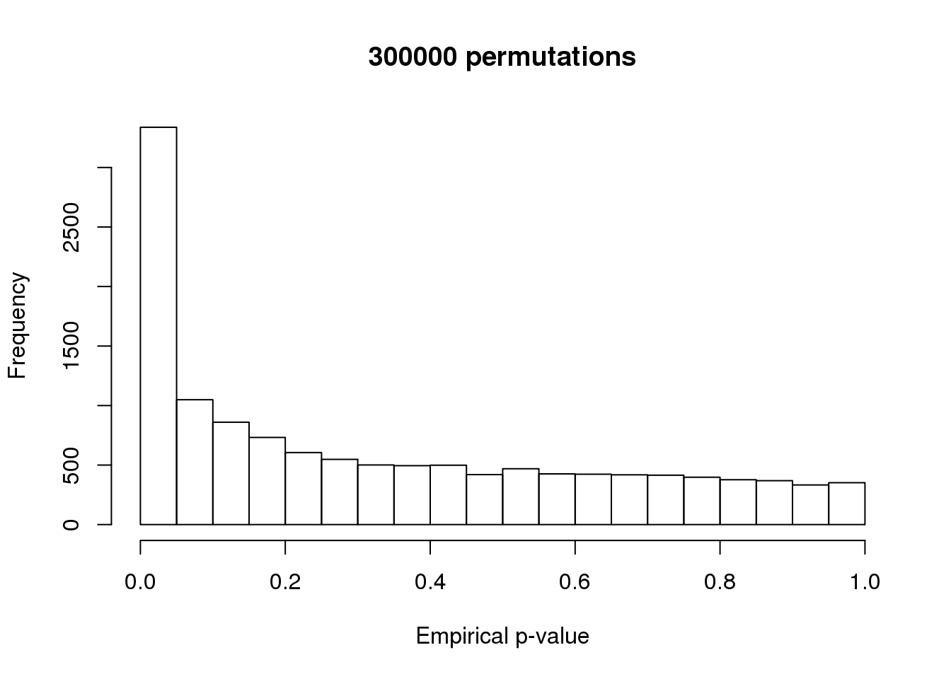
[chunk not evaluated]
# This is an example script used to compute permutation-based MAD statistic.
library(Humanzee)
perm_set <- do.call(cbind, lapply(1:100, function(i) {
  perms <- permute_cv_test(log2counts = molecules_final_subset,
                subset_matrix = molecules_expressed_subset,
                grouping_vector = anno_filter$individual,
                anno = anno_filter,
                number_permute = 10,
                output_rda = FALSE,
                do_parallel = TRUE,
                number_cores = 8)
  return(perms)
})  )
save(perm_set,
     file = "rda/cv-adjusted-summary-pois-expressed/mad-perm-values.rda")

# table(c(rowSums(perm_data > mad_expressed)) > 0)
# perm_pval <- (rowSums(perm_set > mad_expressed) + 1)/( NCOL(perm_set) + 1)
# hist(perm_pval)
# perm_fdr <- p.adjust(perm_pval, method = "fdr")
# summary(perm_fdr)
# sum(perm_fdr < .01, na.rm = TRUE)
Pluripotency genes
*P < .0001
sig_genes <- names(perm_pval_set1)[which(perm_pval_set1 < .0001)]
sig_genes[which(sig_genes %in% pluripotency_genes)]
[1] "ENSG00000163530" "ENSG00000136826"gene_symbols[which(gene_symbols$ensembl_gene_id %in% sig_genes[which(sig_genes %in% pluripotency_genes)]), ] ensembl_gene_id chromosome_name external_gene_name transcript_count
5686 ENSG00000136826 9 KLF4 5
8354 ENSG00000163530 3 DPPA2 1
description
5686 Kruppel-like factor 4 (gut) [Source:HGNC Symbol;Acc:6348]
8354 developmental pluripotency associated 2 [Source:HGNC Symbol;Acc:19197]Print out pluripotent genes
sig_pluri_ensg <- gene_symbols[which(gene_symbols$ensembl_gene_id %in% sig_genes[which(sig_genes %in% pluripotency_genes)]), ]

source("../code/plotting-functions.R")
par(mfrow = c(1,2))
for (i in 1:length(sig_pluri_ensg$ensembl_gene_id)) {
  plot_density_overlay(
    molecules = molecules_final_expressed_subset,
    annotation = anno_filter,
    which_gene = sig_pluri_ensg$ensembl_gene_id[i],
    labels = "",
#    xlims = c(8,15),
#    ylims = c(0,1.5),
    cex.lab = 1.2,
    cex.axis = 1.2,
    gene_symbols = gene_symbols)
}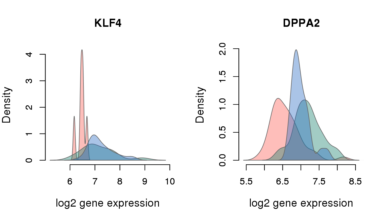
pvals <- perm_pval_set1[which(names(perm_pval_set1) %in% sig_pluri_ensg$ensembl_gene_id)]
cbind(pvals,
      mad_expressed[match(names(pvals), names(perm_pval_set1))],
      gene_symbols$external_gene_name[match(names(pvals), gene_symbols$ensembl_gene_id)])
pvals
ENSG00000163530 "3.33332222225926e-06" "0.254282140102765" "DPPA2"
ENSG00000136826 "3.33332222225926e-06" "0.340412425324323" "KLF4" for (i in 1:2) {
print(sig_pluri_ensg$external_gene_name[i])
print(table(molecules_expressed_subset[rownames(molecules_expressed_subset) %in% sig_pluri_ensg$ensembl_gene_id[i]], anno_filter$individual) )
}[1] "KLF4"
NA19098 NA19101 NA19239
0 136 187 189
1 6 14 32
[1] "DPPA2"
NA19098 NA19101 NA19239
0 95 168 197
1 47 33 24Enrichment analysis of differential CV genes
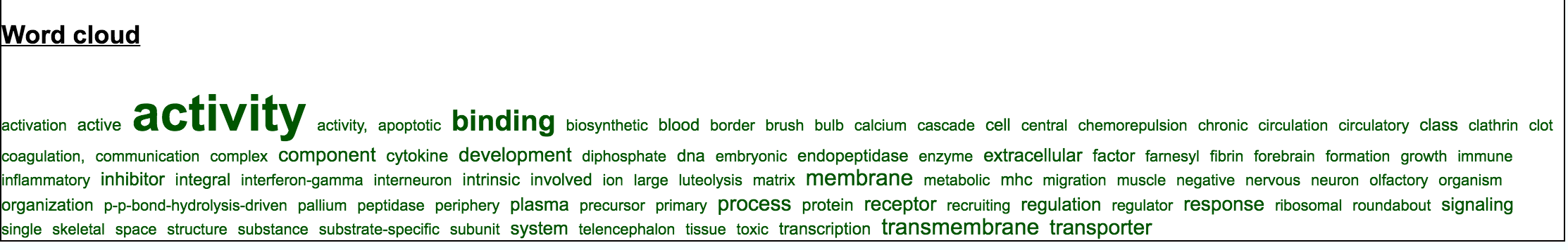
I used CPDB (http://cpdb.molgen.mpg.de/) for over-representation gene set enrichment analysis. The enriched GO term are represented in WordCloud as follows.
Supplemental tables for the manuscript
Supplemental Table 2: Significant inter-individual variation genes
Output signficant genes
sig_genes <- names(perm_pval_set1)[which(perm_pval_set1 < .0001)]
sig_genes_output <-
  data.frame(ensg = sig_genes,
             symbol = gene_symbols$external_gene_name[which(gene_symbols$ensembl_gene_id %in% sig_genes)],
             permute_pval = perm_pval_set1[which(perm_pval_set1 < .0001)])

write.table(sig_genes_output[order(sig_genes_output$permute_pval),],
            quote = FALSE,
            col.names = FALSE,
            row.names = FALSE,
            sep = "\t",
            file = "../data/sig-expressed-genes.txt")
Supplemental Table 3: Gene ontology over-representation analysis for significant genes
"figure/cv-adjusted-summary-pois-expressed.Rmd/go-expressed-sig-xls"Session information
sessionInfo()R version 3.2.0 (2015-04-16)
Platform: x86_64-unknown-linux-gnu (64-bit)
locale:
[1] LC_CTYPE=en_US.UTF-8 LC_NUMERIC=C
[3] LC_TIME=en_US.UTF-8 LC_COLLATE=en_US.UTF-8
[5] LC_MONETARY=en_US.UTF-8 LC_MESSAGES=en_US.UTF-8
[7] LC_PAPER=en_US.UTF-8 LC_NAME=C
[9] LC_ADDRESS=C LC_TELEPHONE=C
[11] LC_MEASUREMENT=en_US.UTF-8 LC_IDENTIFICATION=C
attached base packages:
[1] stats4 parallel grid stats graphics grDevices utils
[8] datasets methods base
other attached packages:
[1] broman_0.59-5 scales_0.4.0 gridExtra_2.0.0
[4] VennDiagram_1.6.9 mygene_1.2.3 GenomicFeatures_1.20.1
[7] AnnotationDbi_1.30.1 Biobase_2.28.0 GenomicRanges_1.20.5
[10] GenomeInfoDb_1.4.0 IRanges_2.2.4 S4Vectors_0.6.0
[13] BiocGenerics_0.14.0 matrixStats_0.14.0 MASS_7.3-40
[16] cowplot_0.3.1 Humanzee_0.1.0 ggplot2_1.0.1
[19] knitr_1.10.5
loaded via a namespace (and not attached):
[1] Rcpp_0.12.4 lattice_0.20-31
[3] Rsamtools_1.20.4 Biostrings_2.36.1
[5] assertthat_0.1 digest_0.6.8
[7] plyr_1.8.3 chron_2.3-45
[9] futile.options_1.0.0 acepack_1.3-3.3
[11] RSQLite_1.0.0 evaluate_0.7
[13] httr_0.6.1 sqldf_0.4-10
[15] zlibbioc_1.14.0 rpart_4.1-9
[17] rmarkdown_0.6.1 gsubfn_0.6-6
[19] proto_0.3-10 labeling_0.3
[21] splines_3.2.0 BiocParallel_1.2.2
[23] stringr_1.0.0 foreign_0.8-63
[25] RCurl_1.95-4.6 biomaRt_2.24.0
[27] munsell_0.4.3 rtracklayer_1.28.4
[29] htmltools_0.2.6 nnet_7.3-9
[31] Hmisc_3.16-0 XML_3.98-1.2
[33] GenomicAlignments_1.4.1 bitops_1.0-6
[35] jsonlite_0.9.16 gtable_0.1.2
[37] DBI_0.3.1 magrittr_1.5
[39] formatR_1.2 stringi_1.0-1
[41] XVector_0.8.0 reshape2_1.4.1
[43] latticeExtra_0.6-26 futile.logger_1.4.1
[45] Formula_1.2-1 lambda.r_1.1.7
[47] RColorBrewer_1.1-2 tools_3.2.0
[49] survival_2.38-1 yaml_2.1.13
[51] colorspace_1.2-6 cluster_2.0.1