Quality control plots
PoYuan Tung
2015-10-21
Last updated: 2016-11-08
Code version: bd286a36f14d3b332285cdc7e62258b1f616bb14
Input
library("biomaRt")
library("data.table")
library("dplyr")
library("limma")
library("edgeR")
library("ggplot2")
library("grid")
library("cowplot")
theme_set(theme_bw(base_size = 16))
theme_update(panel.grid.minor.x = element_blank(),
             panel.grid.minor.y = element_blank(),
             panel.grid.major.x = element_blank(),
             panel.grid.major.y = element_blank(),
             legend.key = element_blank(),
             plot.title = element_text(size = rel(1)))
source("functions.R")
Input ERCC molecule counts calculated in capture efficiency.
ercc <- read.table("../data/expected-ercc-molecules.txt", header = TRUE,
                   stringsAsFactors = FALSE)
head(ercc)
id conc_mix1 ercc_molecules_well
1 ERCC-00130 30000.000 4877.93485
2 ERCC-00004 7500.000 1219.48371
3 ERCC-00136 1875.000 304.87093
4 ERCC-00108 937.500 152.43546
5 ERCC-00116 468.750 76.21773
6 ERCC-00092 234.375 38.10887Input annotation.
anno <- read.table("../data/annotation.txt", header = TRUE,
                   stringsAsFactors = FALSE)
head(anno)
individual replicate well batch sample_id
1 NA19098 r1 A01 NA19098.r1 NA19098.r1.A01
2 NA19098 r1 A02 NA19098.r1 NA19098.r1.A02
3 NA19098 r1 A03 NA19098.r1 NA19098.r1.A03
4 NA19098 r1 A04 NA19098.r1 NA19098.r1.A04
5 NA19098 r1 A05 NA19098.r1 NA19098.r1.A05
6 NA19098 r1 A06 NA19098.r1 NA19098.r1.A06Input read counts and filter for quality cells.
reads <- read.table("../data/reads.txt", header = TRUE,
                    stringsAsFactors = FALSE)

quality_single_cells <- scan("../data/quality-single-cells.txt", what = "character")
reads <- reads[, colnames(reads) %in% quality_single_cells]
Input read counts in high quality cells for filtered genes
reads_filter <- read.table("../data/reads-filter.txt", header = TRUE,
                    stringsAsFactors = FALSE)
Input molecule counts and filter for quality cell.
molecules <- read.table("../data/molecules.txt", header = TRUE,
                    stringsAsFactors = FALSE)

molecules <- molecules[, colnames(molecules) %in% quality_single_cells]
Input molecule counts in high quality cells for filtered genes
molecules_filter <- read.table("../data/molecules-filter.txt", header = TRUE,
                    stringsAsFactors = FALSE)
Compare reads and molecules
Compare the means of each gene obtained via the different methods.
## calculate mean
reads_mean     <- apply(reads, 1, mean)
molecules_mean <- apply(molecules, 1, mean)
distribution <- data.frame(reads_mean, molecules_mean)

reads_filter_mean <- apply(reads_filter, 1, mean)
molecules_filter_mean <- apply(molecules_filter, 1, mean)
distribution_filter <- data.frame(reads_filter_mean, molecules_filter_mean)

## correlation between reads and molecules
cor(distribution)
reads_mean molecules_mean
reads_mean 1.0000000 0.9277703
molecules_mean 0.9277703 1.0000000cor(distribution_filter) reads_filter_mean molecules_filter_mean
reads_filter_mean 1.0000000 0.9408234
molecules_filter_mean 0.9408234 1.0000000## select ERCC
distribution$type <- ifelse(grepl("ERCC", rownames(distribution)), "ERCC", "gene")
distribution_filter$type <- ifelse(grepl("ERCC", rownames(distribution_filter)), "ERCC", "gene")
## color palette
cbPalette <- c("#0000FF", "#999999", "#990033", "#F0E442", "#0072B2", "#D55E00", "#CC79A7", "#009E73")
## plots
plot_mean_log <- ggplot(distribution, aes(x = molecules_mean, y = reads_mean, col = type)) +
geom_point(size = 3, alpha = 0.5) +
scale_colour_manual(values=cbPalette) +
labs(x = "Mean molecule-counts across samples",
y = "Mean read-counts across samples",
title = "Amplification bias is stronger \n in endogenous genes than in ERCC spike-ins") +
scale_x_log10() +
scale_y_log10()
plot_mean_log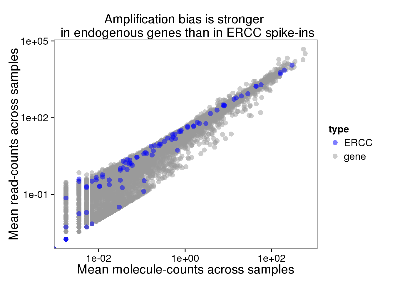
plot_mean_filter_log <- ggplot(distribution_filter, aes(x = molecules_filter_mean, y = reads_filter_mean, col = type)) +
  geom_point(size = 3, alpha = 0.5) +
  scale_colour_manual(values=cbPalette) +
  labs(x = "Mean molecule-counts across samples",
       y = "Mean read-counts",
       title = "Read-counts and molecule-counts of each gene (log scale)") +
  scale_x_log10() +
  scale_y_log10()

plot_mean_filter_log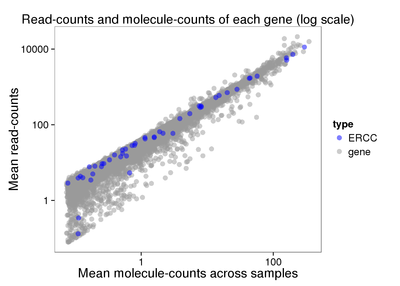
plot_mean <- ggplot(distribution, aes(x = molecules_mean, y = reads_mean, col = type)) +
  geom_point(size = 3, alpha = 0.5) +
  scale_colour_manual(values=cbPalette) +
  labs(x = "Mean molecule-counts across samples",
       y = "Mean read-counts across samples",
       title = "Amplification bias is stronger \n in endogenous genes than in ERCC spike-ins") +
  geom_smooth(method = "lm")

plot_mean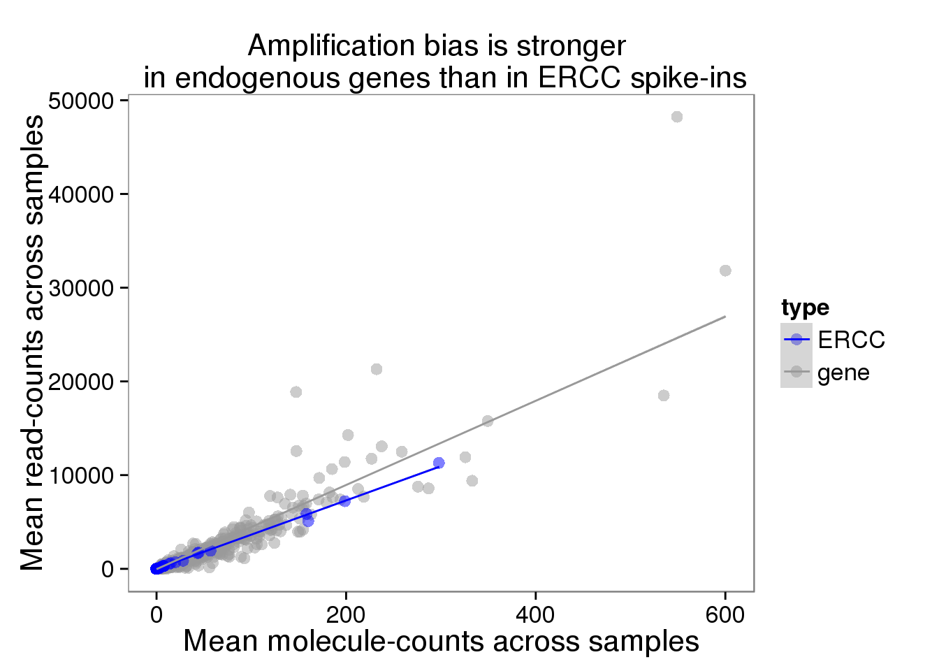
Distribution of fold change to mean
Look at the distribution of fold change to mean. As being reported by others, the lowly expressed genes show divergent read and molecule counts
## calculate fold change to mean
distribution$fold_change_read     <- log2(reads_mean/mean(reads_mean))
distribution$fold_change_molecule <- log2(molecules_mean/mean(molecules_mean))

plot_distribution <- ggplot(distribution, aes(x = fold_change_molecule, y = fold_change_read, col = type)) +
  geom_point(size = 3, alpha = 0.5) +
  scale_colour_manual(values=cbPalette) +
  stat_function(fun= function(x) {x}, col= "#56B4E9") +
  labs(x = "log2 fold change to mean (molecule)", y =  "log2 fold change to mean (reads)")

plot_distribution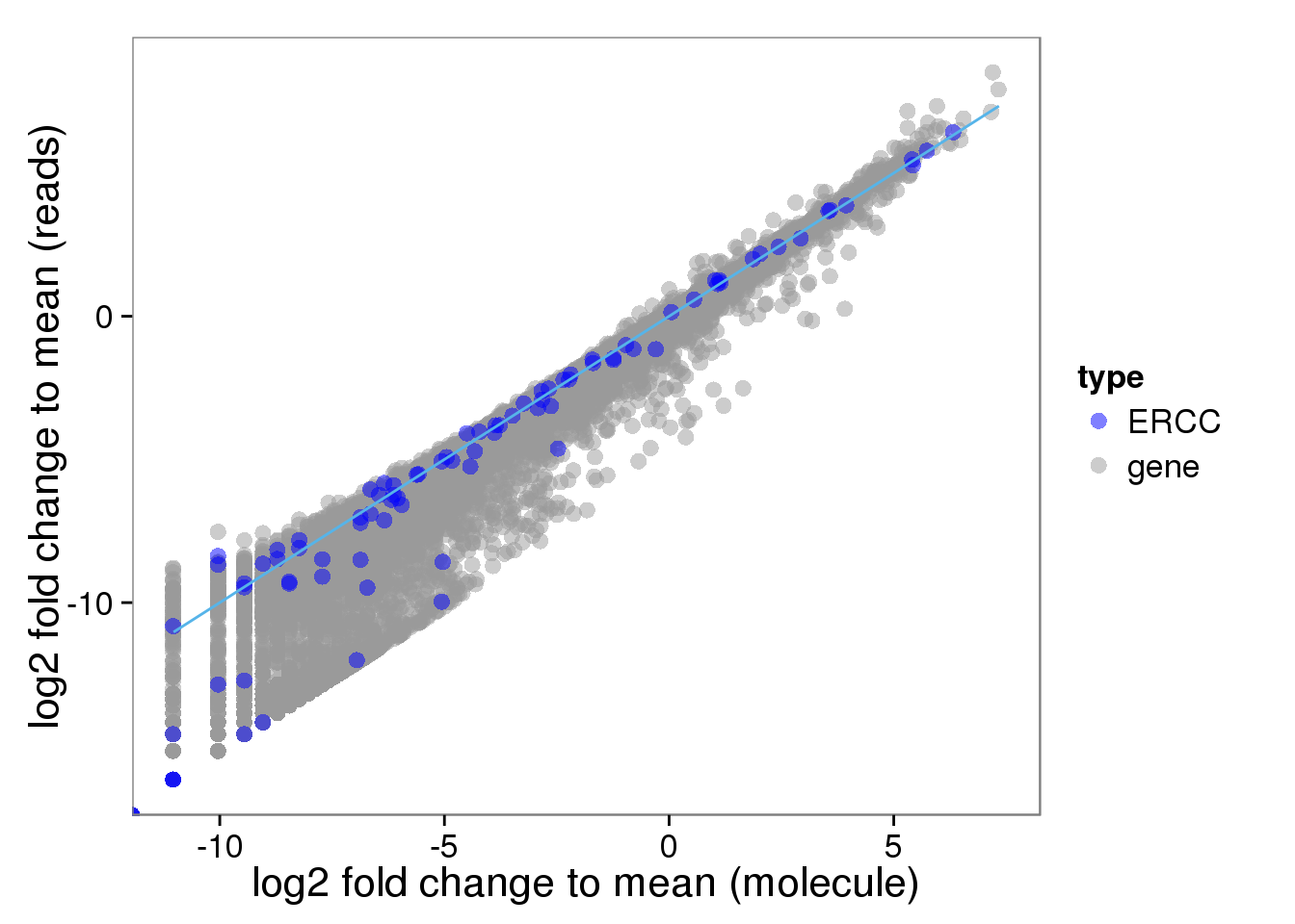
Visualizing capture efficiency
Use only those 50 ERCC genes with at least 1 expected molecule per well.
ercc_list <- list()
for (spike in ercc$id[ercc$ercc_molecules_well >= 1]) {
  if (spike %in% rownames(molecules)) {
    ercc_list$id <- c(ercc_list$id, spike)
    ercc_list$observed_mean <- c(ercc_list$observed_mean,
                                 mean(as.numeric(molecules[spike, ])))
    ercc_list$observed_sem <- c(ercc_list$observed_sem,
                                 sd(as.numeric(molecules[spike, ])) /
                                 sqrt(ncol(molecules)))
    ercc_list$expected <- c(ercc_list$expected,
                            ercc$ercc_molecules_well[ercc$id == spike])
  }
}
ercc_plot <- as.data.frame(ercc_list, stringsAsFactors = FALSE)
str(ercc_plot)
'data.frame': 50 obs. of 4 variables:
$ id : chr "ERCC-00130" "ERCC-00004" "ERCC-00136" "ERCC-00108" ...
$ observed_mean: num 298.1879 57.2784 20.1933 13.5833 0.0603 ...
$ observed_sem : num 2.8448 0.6346 0.2841 0.2141 0.0106 ...
$ expected : num 4877.9 1219.5 304.9 152.4 76.2 ...cor(ercc_plot$observed_mean, ercc_plot$expected)[1] 0.9916157Use molecule filter file.
ercc_list_filter <- list()
for (spike in ercc$id[ercc$ercc_molecules_well >= 0]) {
  if (spike %in% rownames(molecules_filter)) {
    ercc_list_filter$id <- c(ercc_list_filter$id, spike)
    ercc_list_filter$observed_mean <- c(ercc_list_filter$observed_mean,
                                 mean(as.numeric(molecules_filter[spike, ])))
    ercc_list_filter$observed_sem <- c(ercc_list_filter$observed_sem,
                                 sd(as.numeric(molecules_filter[spike, ])) /
                                 sqrt(ncol(molecules_filter)))
    ercc_list_filter$expected <- c(ercc_list_filter$expected,
                            ercc$ercc_molecules_well[ercc$id == spike])
  }
}
ercc_filter_plot <- as.data.frame(ercc_list_filter, stringsAsFactors = FALSE)
str(ercc_filter_plot)
'data.frame': 48 obs. of 4 variables:
$ id : chr "ERCC-00130" "ERCC-00004" "ERCC-00136" "ERCC-00108" ...
$ observed_mean: num 298.19 57.28 20.19 13.58 2.15 ...
$ observed_sem : num 2.8448 0.6346 0.2841 0.2141 0.0674 ...
$ expected : num 4877.9 1219.5 304.9 152.4 38.1 ...cor(ercc_filter_plot$observed_mean, ercc_filter_plot$expected)[1] 0.9916498p_efficiency <- ggplot(ercc_plot, aes(x = expected, y = observed_mean, label = id)) +
geom_point(col = "red") +
geom_errorbar(aes(ymin = observed_mean - observed_sem,
ymax = observed_mean + observed_sem), width = 0) +
labs(x = "Expected ERCC molecules",
y = "Observed ERCC molecules\n(mean +/- SEM)",
title = "ERCC capture efficiency")
p_efficiency_plot <- p_efficiency + scale_x_log10() +
scale_y_log10() +
labs(x = "Expected ERCC molecules",
y = "Observed ERCC molecules\n(mean +/- SEM)",
title = "ERCC capture efficiency \n (48 ERCC spike-in controls)")
p_efficiency_plot + geom_text(hjust = 0, nudge_x = 0.05, size = 4)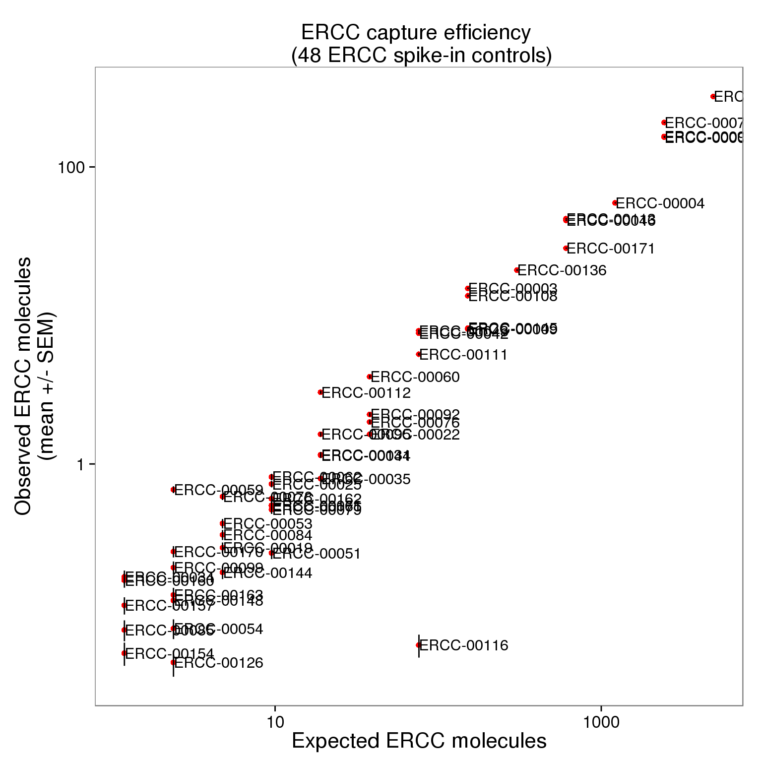
p_efficiency_filter_plot <- ggplot(ercc_filter_plot, aes(x = expected, y = observed_mean)) +
  geom_point(col = "red") +
  geom_errorbar(aes(ymin = observed_mean - observed_sem,
                    ymax = observed_mean + observed_sem), width = 0) +
                    scale_x_log10() + scale_y_log10() +
                    labs(x = "Expected ERCC molecules",
                    y = "Observed ERCC molecules\n(mean +/- SEM)",
                    title = "ERCC capture efficiency")

p_efficiency_filter_plot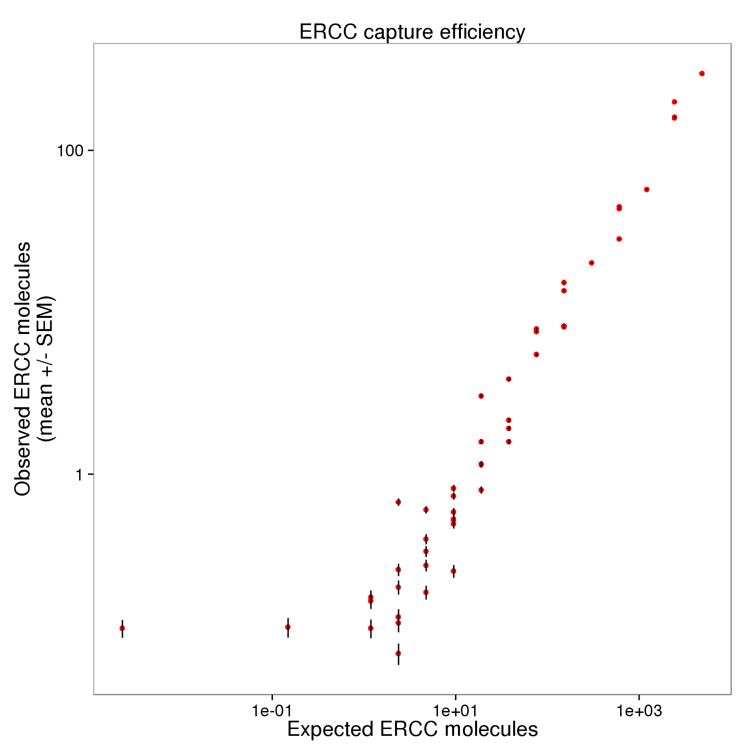
Calculate capture efficiency per cell
ercc_index <- grep("ERCC", rownames(molecules_filter))
length(ercc_index)
[1] 48efficiency <- numeric(length = ncol(molecules_filter))
total_ercc_molecules <- sum(ercc_filter_plot$expected)
for (i in 1:ncol(molecules_filter)) {
efficiency[i] <- sum(molecules_filter[ercc_index, i]) / total_ercc_molecules
}
summary(efficiency) Min. 1st Qu. Median Mean 3rd Qu. Max.
0.03978 0.05459 0.06140 0.06580 0.07621 0.12150 QC plots for paper
plot_grid(plot_mean_log + theme(legend.position = c(.85,.25)) + labs (col = ""),
          p_efficiency_plot + theme(legend.position = "none"),
          labels = letters[6:7])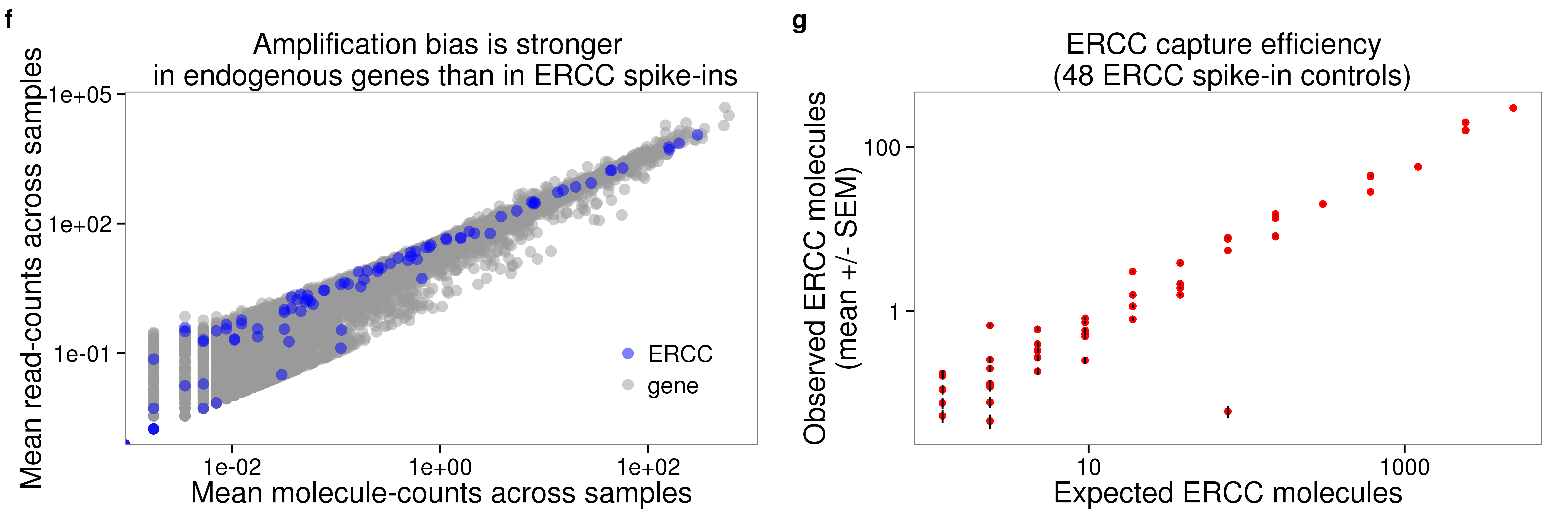
Session information
sessionInfo()R version 3.2.0 (2015-04-16)
Platform: x86_64-unknown-linux-gnu (64-bit)
locale:
[1] LC_CTYPE=en_US.UTF-8 LC_NUMERIC=C
[3] LC_TIME=en_US.UTF-8 LC_COLLATE=en_US.UTF-8
[5] LC_MONETARY=en_US.UTF-8 LC_MESSAGES=en_US.UTF-8
[7] LC_PAPER=en_US.UTF-8 LC_NAME=C
[9] LC_ADDRESS=C LC_TELEPHONE=C
[11] LC_MEASUREMENT=en_US.UTF-8 LC_IDENTIFICATION=C
attached base packages:
[1] grid stats graphics grDevices utils datasets methods
[8] base
other attached packages:
[1] cowplot_0.3.1 ggplot2_1.0.1 edgeR_3.10.2 limma_3.24.9
[5] dplyr_0.4.2 data.table_1.9.4 biomaRt_2.24.0 knitr_1.10.5
loaded via a namespace (and not attached):
[1] Rcpp_0.12.4 formatR_1.2 GenomeInfoDb_1.4.0
[4] plyr_1.8.3 bitops_1.0-6 tools_3.2.0
[7] digest_0.6.8 RSQLite_1.0.0 evaluate_0.7
[10] gtable_0.1.2 DBI_0.3.1 yaml_2.1.13
[13] parallel_3.2.0 proto_0.3-10 httr_0.6.1
[16] stringr_1.0.0 S4Vectors_0.6.0 IRanges_2.2.4
[19] stats4_3.2.0 Biobase_2.28.0 R6_2.1.1
[22] AnnotationDbi_1.30.1 XML_3.98-1.2 rmarkdown_0.6.1
[25] reshape2_1.4.1 magrittr_1.5 scales_0.4.0
[28] htmltools_0.2.6 BiocGenerics_0.14.0 MASS_7.3-40
[31] assertthat_0.1 colorspace_1.2-6 labeling_0.3
[34] stringi_1.0-1 RCurl_1.95-4.6 munsell_0.4.3
[37] chron_2.3-45