parametric cellcycleR for image intensities: convergence assessment

Introduction/Summary

In this document, we assess the convergence of cellcycleR across all samples and all batches on fitting intensity data - three intensity vectors for ~1,200 single cell samples.

Results:

20 runs of sin_cell_ordering_class on 20 different random seeds. Each 500 iterations. We assess the range of log-likelihood, and model estimates \(\hat{\alpha}_g\), \(\hat{\phi}_g\), and \(\hat{\sigma}_g\).

1. Large deviation in the estimates of \(\phi_g\): because \(\phi_g\) is not identifiable.

2. Not much deviation between the 20 runs in the estimates for \(\alpha_g\) amplitude or \(\sigma_g\) or log-likelihood.

3. Re. speed of convergence, across random seeds, it takes about less than 50 iterations to reach convergence. Note that the observation vector of each cell is a three-dimensional vector (green, red, and dapi). The number of iterations will go up as we increase the dimension of the observations (e.g., number of genes).

Data

Combined intensity data (see combine-intensity-data.R).

Model overview

For \(S\) cells, let the vector of true cell time be \(t_S\). We use an iterative scheme to estimate cell time parameters \(t_S\), and curve parameters \(\alpha_g\), \(\phi_g\), and \(\sigma_g\). First, we consider \(T\) time classes which is a set of uniformly spaced time points on \((0, 2\pi)\). In the first iteration, we assign each cell \(s\) to a time class \(t_s^{(0)}\) and estimate the curve parameters \(\alpha_g\), \(\phi_g\), and \(\sigma_g\). In the second iteratio, we estimate \(t_s^{(1)}\) based on the model estimates from the first iteration (\(\hat{\alpha}_g\), \(\hat{\phi}_g\), and \(\hat{\sigma}_g\)). We continue this iterative scheme until convergence. For any \(n\) iterations, starting from 0, we fit the following model for gene \(g\) and and cell \(s\).

\[ Y_{sg} = \alpha_g sin(t_s^{(n)} + \phi_g) + \epsilon_{sg} \] where \(\epsilon_{sg} \sim N(0, \sigma^2_g)\), and frequency is 1.

Analysis

20 runs of sin_cell_ordering_class on 20 different random seeds. Each 500 iterations.

We assess the range of log-likelihood, and model estimates \(\hat{\alpha}_g\), \(\hat{\phi}_g\), and \(\hat{\sigma}_g\).

summary(loglik)

   Min. 1st Qu.  Median    Mean 3rd Qu.    Max. 
  -3350   -3312   -3290   -3290   -3262   -3244 

summary(amp)

      Red            Green            DAPI      
 Min.   :1.289   Min.   :1.060   Min.   :1.002  
 1st Qu.:1.301   1st Qu.:1.081   1st Qu.:1.019  
 Median :1.318   Median :1.093   Median :1.036  
 Mean   :1.316   Mean   :1.090   Mean   :1.035  
 3rd Qu.:1.324   3rd Qu.:1.099   3rd Qu.:1.047  
 Max.   :1.346   Max.   :1.106   Max.   :1.068  

summary(phi)

      Red             Green             DAPI        
 Min.   :0.4663   Min.   :0.1580   Min.   :0.06544  
 1st Qu.:1.2966   1st Qu.:0.6726   1st Qu.:0.64207  
 Median :3.9793   Median :3.4906   Median :3.48495  
 Mean   :3.5329   Mean   :2.9224   Mean   :2.89855  
 3rd Qu.:5.4010   3rd Qu.:4.5465   3rd Qu.:4.47567  
 Max.   :5.9765   Max.   :6.1127   Max.   :6.01985  

summary(sigma)

      Red             Green             DAPI       
 Min.   :0.3654   Min.   :0.6702   Min.   :0.6928  
 1st Qu.:0.3774   1st Qu.:0.6745   1st Qu.:0.7085  
 Median :0.3854   Median :0.6814   Median :0.7141  
 Mean   :0.3876   Mean   :0.6815   Mean   :0.7133  
 3rd Qu.:0.3971   3rd Qu.:0.6873   3rd Qu.:0.7180  
 Max.   :0.4120   Max.   :0.6990   Max.   :0.7230  

log-liklihood distribution

plot(loglik)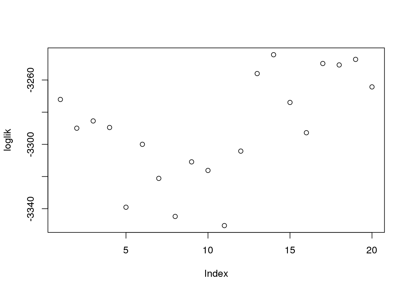

par(mfrow=c(5,4), mar=c(1,1,2.5,1), oma=rep(1,4))
for (i in 1:length(objs)) {
plot(objs[[i]]$loglik_iter[-1],
     main = paste("round no.", i))
}
title("log-likelihood", outer=TRUE)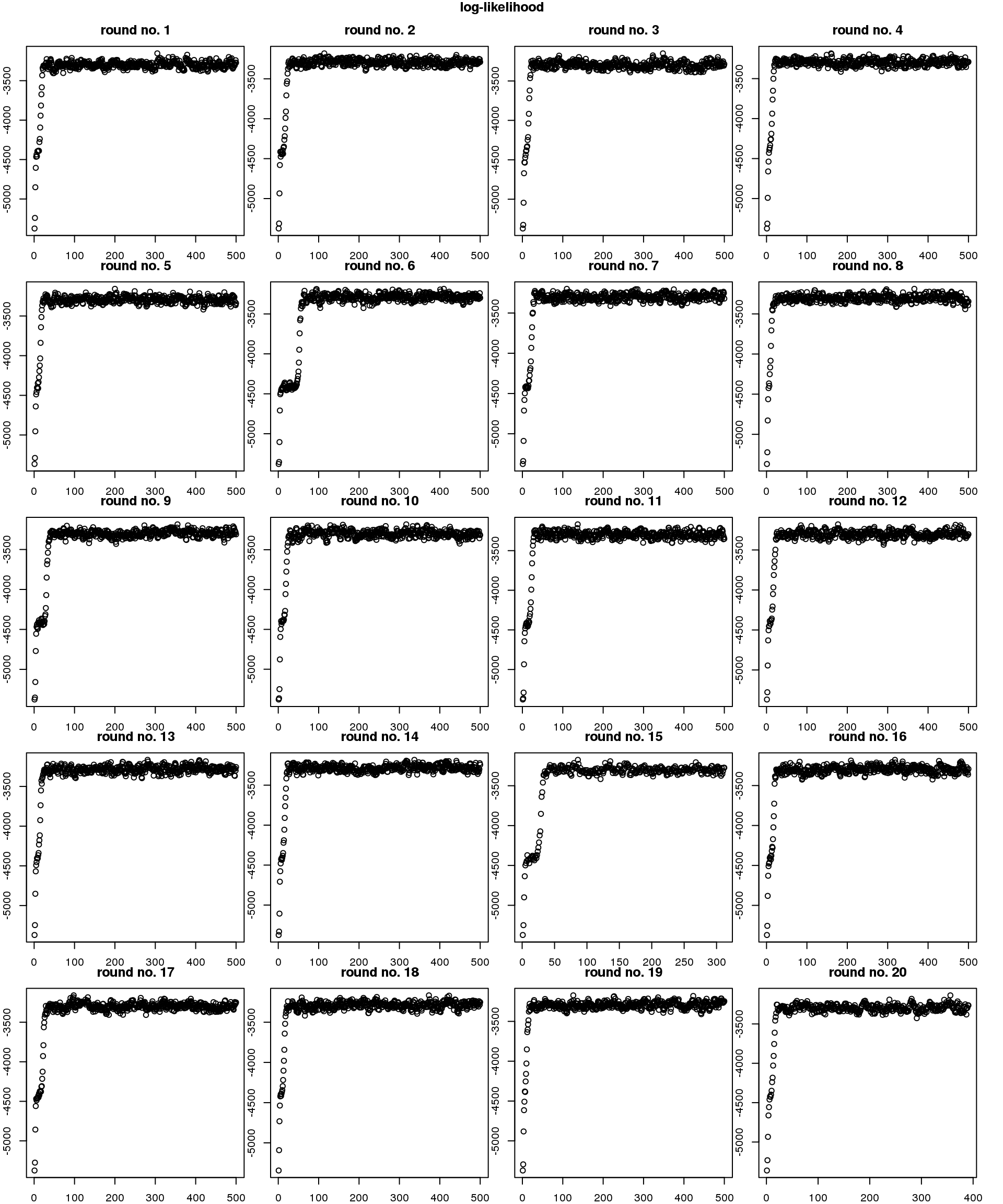

speed of convergence

maxiter <- vector("numeric", length(objs))
for (i in 1:length(maxiter)) {
  maxiter[i] <- which.max(objs[[i]]$loglik_iter[-1]) 
}

boxplot(maxiter, outpch = NA, main = "no. iterations reached for convergence") 
stripchart(maxiter,  
            vertical = TRUE, method = "jitter", 
            pch = 21, col = "maroon", bg = "bisque", 
            add = TRUE)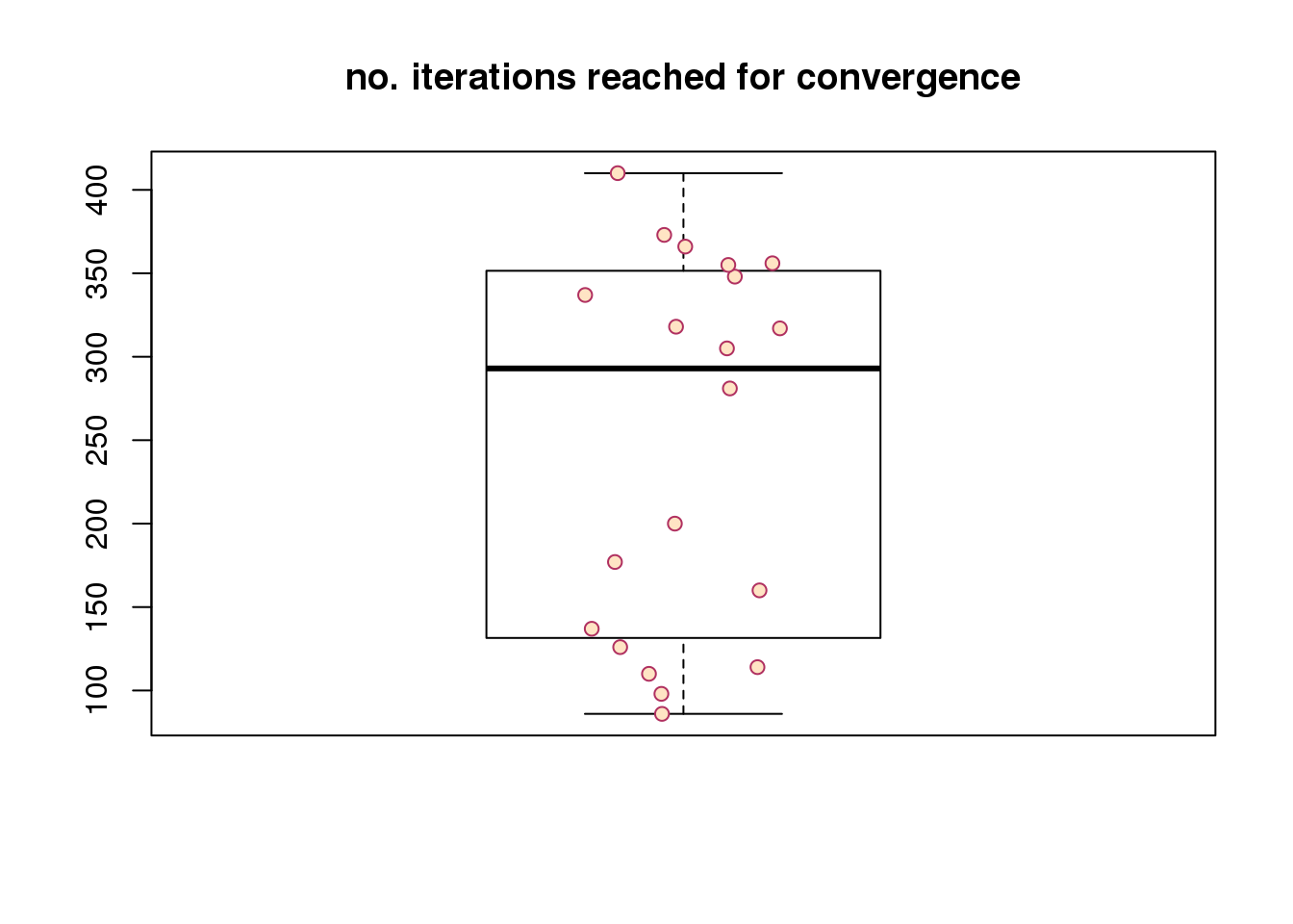 

Session information

R version 3.4.1 (2017-06-30)
Platform: x86_64-redhat-linux-gnu (64-bit)
Running under: Scientific Linux 7.2 (Nitrogen)

Matrix products: default
BLAS/LAPACK: /usr/lib64/R/lib/libRblas.so

locale:
 [1] LC_CTYPE=en_US.UTF-8       LC_NUMERIC=C              
 [3] LC_TIME=en_US.UTF-8        LC_COLLATE=en_US.UTF-8    
 [5] LC_MONETARY=en_US.UTF-8    LC_MESSAGES=en_US.UTF-8   
 [7] LC_PAPER=en_US.UTF-8       LC_NAME=C                 
 [9] LC_ADDRESS=C               LC_TELEPHONE=C            
[11] LC_MEASUREMENT=en_US.UTF-8 LC_IDENTIFICATION=C       

attached base packages:
[1] parallel  stats     graphics  grDevices utils     datasets  methods  
[8] base     

other attached packages:
 [1] plotrix_3.7         Biobase_2.38.0      BiocGenerics_0.24.0
 [4] RColorBrewer_1.1-2  wesanderson_0.3.4   cowplot_0.9.2      
 [7] dplyr_0.7.4         data.table_1.10.4-3 cellcycleR_0.1.6   
[10] zoo_1.8-1           binhf_1.0-1         adlift_1.3-3       
[13] EbayesThresh_1.4-12 wavethresh_4.6.8    MASS_7.3-47        
[16] ggplot2_2.2.1      

loaded via a namespace (and not attached):
 [1] Rcpp_0.12.14     compiler_3.4.1   git2r_0.20.0     plyr_1.8.4      
 [5] bindr_0.1        tools_3.4.1      digest_0.6.13    evaluate_0.10.1 
 [9] tibble_1.3.4     gtable_0.2.0     lattice_0.20-35  pkgconfig_2.0.1 
[13] rlang_0.1.4      yaml_2.1.16      bindrcpp_0.2     stringr_1.2.0   
[17] knitr_1.17       rprojroot_1.3-1  grid_3.4.1       glue_1.2.0      
[21] R6_2.2.2         rmarkdown_1.8    magrittr_1.5     backports_1.1.2 
[25] scales_0.5.0     htmltools_0.3.6  assertthat_0.2.0 colorspace_1.3-2
[29] stringi_1.1.6    lazyeval_0.2.1   munsell_0.4.3