Circle fit to intensities
Joyce Hsiao
Last updated: 2018-02-23
Code version: f434aa3
Overview/Results
Here we estimate a circle fit on the two-dimensional intensity distriubtion of GFP and RFP.
Data and packages
Packages
library(circular)
library(conicfit)
library(Biobase)
library(dplyr)
library(matrixStats)
library(CorShrink)

source("../code/circle.intensity.fit.R")
Load data
df <- readRDS(file="../data/eset-filtered.rds")
pdata <- pData(df)
fdata <- fData(df)

# select endogeneous genes
counts <- exprs(df)[grep("ENSG", rownames(df)), ]

# log2cpm <- readRDS("../output/seqdata-batch-correction.Rmd/log2cpm.rds")
# log2cpm.adjust <- readRDS("../output/seqdata-batch-correction.Rmd/log2cpm.adjust.rds")

# import corrected intensities
pdata.adj <- readRDS("../output/images-normalize-anova.Rmd/pdata.adj.rds")
Circle fitting
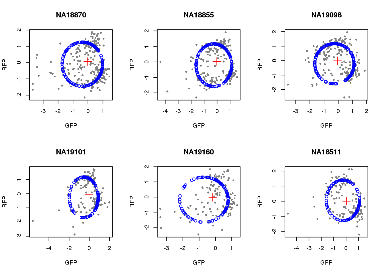
Based on all data.
source("../code/circle.intensity.fit.R")
#sample_names <- rownames(pdata.adj)

pdata.adj <- pdata.adj %>% group_by(chip_id) %>%
  mutate(rfp.z=scale(rfp.median.log10sum.adjust.ash),
            gfp.z=scale(gfp.median.log10sum.adjust.ash),
            dapi.z=scale(dapi.median.log10sum.adjust.ash))
pdata.adj <- data.frame(pdata.adj)

par(mfrow=c(2,3))
for(i in 1:length(unique(pdata.adj$chip_id))) {
  id <- unique(as.character(pdata.adj$chip_id))[i]
  df_sub <- subset(pdata.adj, chip_id == id, select=c(gfp.z, rfp.z))

  cpred <- circle.fit(df_sub)

  xlims <- range(df_sub[,1])
  ylims <- range(df_sub[,2])
  plot(df_sub, pch=16, col="gray50", xlim=xlims, ylim=ylims, cex=.7,
       main = id, xlab="GFP", ylab="RFP")
  points(cpred[,1], cpred[,2], col="blue", type = "p")
  points(mean(cpred[,1]), mean(cpred[,2]), col="red", pch=3, cex=2)
}
Consider deleted residuals.
resids.del <- lapply(1:length(unique(pdata.adj$chip_id)), function(i) {
  id <- unique(as.character(pdata.adj$chip_id))[i]
  df_sub <- subset(pdata.adj, chip_id == id, select=c(gfp.z, rfp.z))
  resids <- circle.fit.resid.delete(df_sub)
  scale(resids)
})
names(resids.del) <- unique(pdata.adj$chip_id)

par(mfrow=c(2,3))
for(i in 1:length(unique(pdata.adj$chip_id))) {
  # id <- unique(as.character(pdata.adj$chip_id))[i]
  # df_sub <- subset(pdata.adj, chip_id == id, select=c(gfp.z, rfp.z))
  hist(resids.del[[i]], main = unique(pdata.adj$chip_id)[i])
}
Remove samples with standardized residuals greater than 3.
resids.del.remove <- lapply(1:length(unique(pdata.adj$chip_id)), function(i) {
which(resids.del[[i]] > 3)
})
names(resids.del.remove) <- unique(pdata.adj$chip_id)
pdata.adj.filt <- do.call(rbind, lapply(1:length(unique(pdata.adj$chip_id)), function(i) {
id <- unique(as.character(pdata.adj$chip_id))[i]
df_sub <- pdata.adj[which(pdata.adj$chip_id == id),]
ii.remove <- resids.del.remove[[i]]
df_sub_return <- df_sub[-ii.remove,]
rownames(df_sub_return) <- (rownames(pdata.adj)[which(pdata.adj$chip_id == id)])[-ii.remove]
data.frame(df_sub_return)
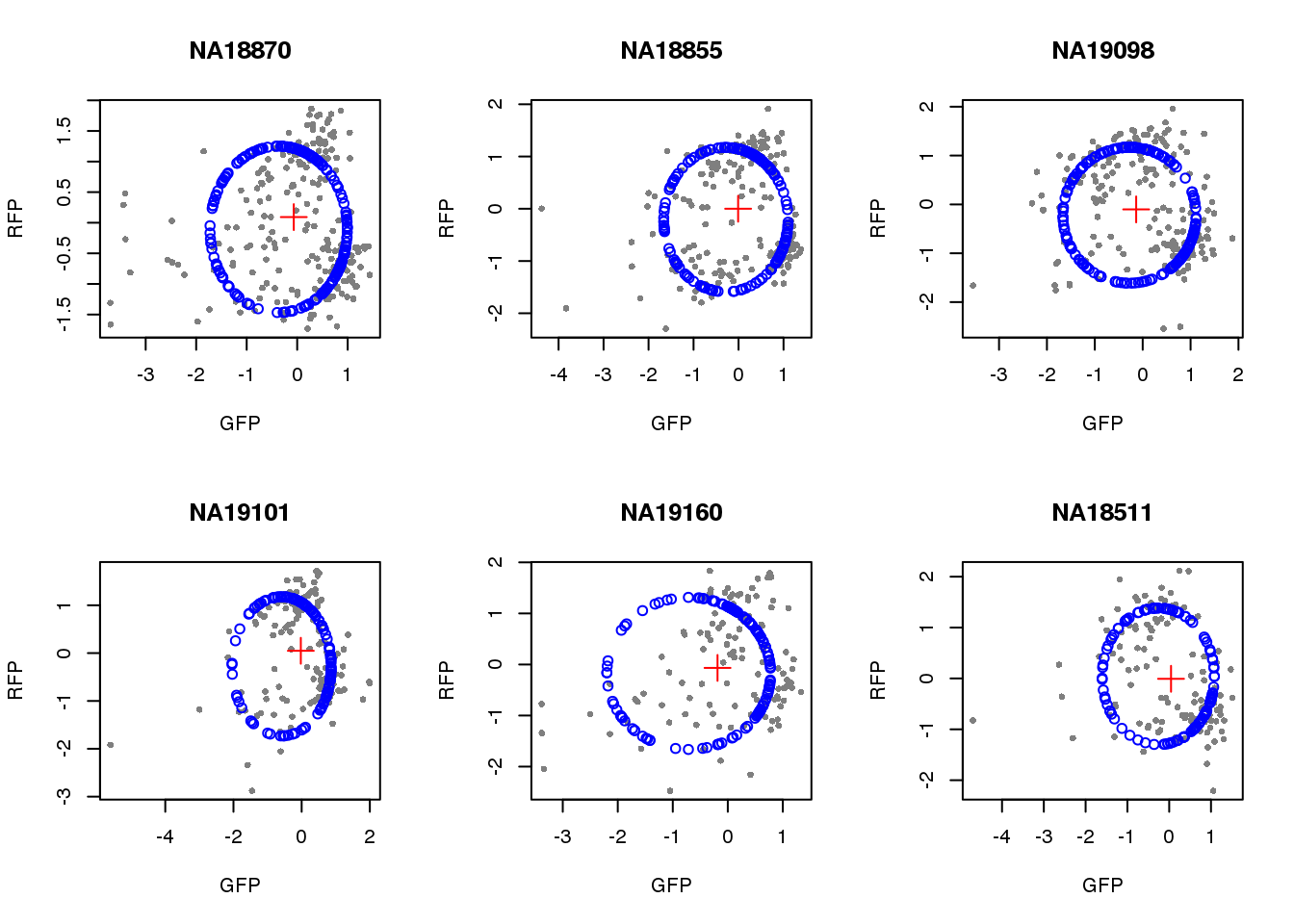
}) )Visualize fit after removing outliers.
par(mfrow=c(2,3))
for(i in 1:length(unique(pdata.adj.filt$chip_id))) {
  id <- unique(as.character(pdata.adj.filt$chip_id))[i]
  df_sub <- subset(pdata.adj.filt, chip_id == id, select=c(gfp.z, rfp.z))

  cpred <- circle.fit(df_sub)

  xlims <- range(df_sub[,1])
  ylims <- range(df_sub[,2])
  plot(df_sub, pch=16, col="gray50", xlim=xlims, ylim=ylims, cex=.7,
       main = id, xlab="GFP", ylab="RFP")
  points(cpred[,1], cpred[,2], col="blue", type = "p")
  points(mean(cpred[,1]), mean(cpred[,2]), col="red", pch=3, cex=2)
}
saveRDS(pdata.adj.filt,
        file = "../output/images-circle-ordering.Rmd/pdata.adj.filt.rds")
Project positions
pdata.adj.filt <- readRDS("../output/images-circle-ordering.Rmd/pdata.adj.filt.rds")

proj.res <- vector("list", length=length(unique((pdata.adj$chip_id))))

for(i in 1:length(unique((pdata.adj$chip_id)))) {
  proj.res[[i]] <- vector("list",2)

  id <- unique(as.character(pdata.adj.filt$chip_id))[i]

  df_sub <- subset(pdata.adj.filt,
                   chip_id == id, select=c(gfp.z, rfp.z))
#  sample_ids <-

  cpred <- circle.fit(df_sub)

  proj.res[[i]][[1]] <- data.frame(cpred, df_sub)
  colnames(proj.res[[i]][[1]]) <- c("pos.pred.x", "pos.pred.y", "gfp.z", "rfp.z")

  # convert projected coordinates to radians
  # modulo 2*pi
  proj.res[[i]][[1]]$rads <- coord2rad(cbind(proj.res[[i]][[1]]$pos.pred.x,
                                        proj.res[[i]][[1]]$pos.pred.y))
  rownames(proj.res[[i]][[1]]) <- rownames(df_sub)

  # compute centers
  centers <- LMcircleFit(as.matrix(df_sub), ParIni=colMeans(as.matrix(df_sub)), IterMAX=50)

  proj.res[[i]][[2]] <- data.frame(x.center=centers[1], y.center=centers[2])
}
names(proj.res) <- unique(pdata.adj.filt$chip_id)
Save output
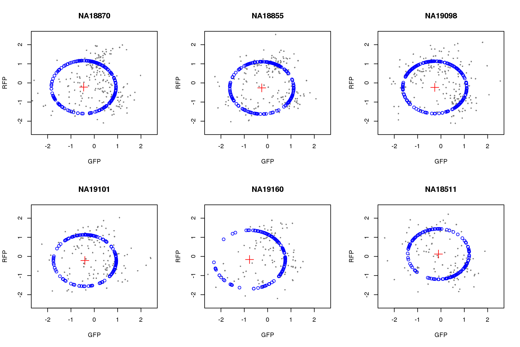
saveRDS(proj.res, file = "../output/images-circle-ordering.Rmd/proj.res.rds")Plot circle fit.
proj.res <- readRDS(file = "../output/images-circle-ordering.Rmd/proj.res.rds")

par(mfrow=c(2,3))
for (i in 1:length(proj.res)) {
  # xlims <- range(proj.res[[i]]$gfp.z)
  # ylims <- range(proj.res[[i]]$rfp.z)
  xlims <- c(-2.5, 2.5)
  ylims <- c(-2.5, 2.5)
  plot(subset(proj.res[[i]][[1]], select=c(gfp.z, rfp.z)),
       pch=16, col="gray50", xlim=xlims, ylim=ylims, cex=.5,
       main = names(proj.res)[i],
       xlab = "GFP", ylab = "RFP")
  points(proj.res[[i]][[1]]$pos.pred.x, proj.res[[i]][[1]]$pos.pred.y,
         col="blue", pch=1)
  points(proj.res[[i]][[2]]$x.center, proj.res[[i]][[2]]$y.center,
         col="red", pch=3, cex=2)
}
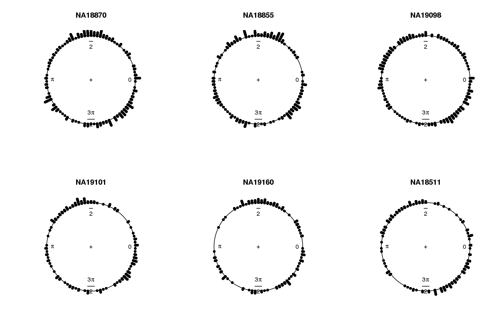
par(mfrow=c(2,3))
for (i in 1:length(proj.res)) {
  plot(proj.res[[i]][[1]]$rads, stack=TRUE, bins=90,
       main = names(proj.res)[i])
}
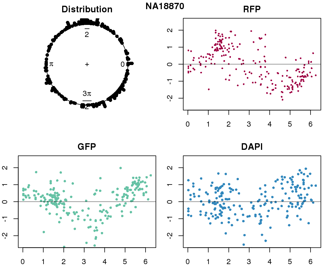
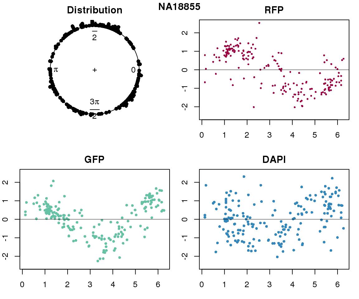
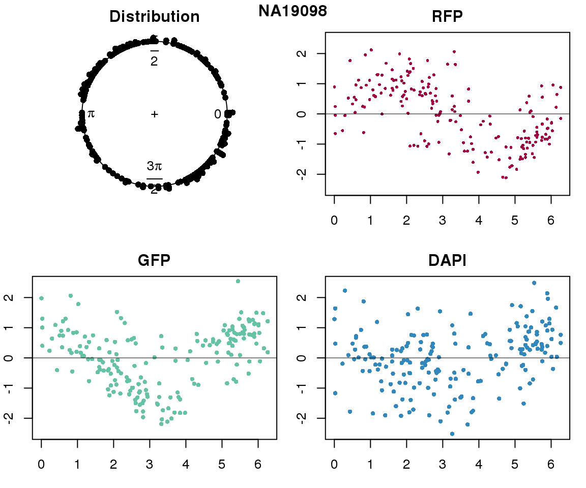
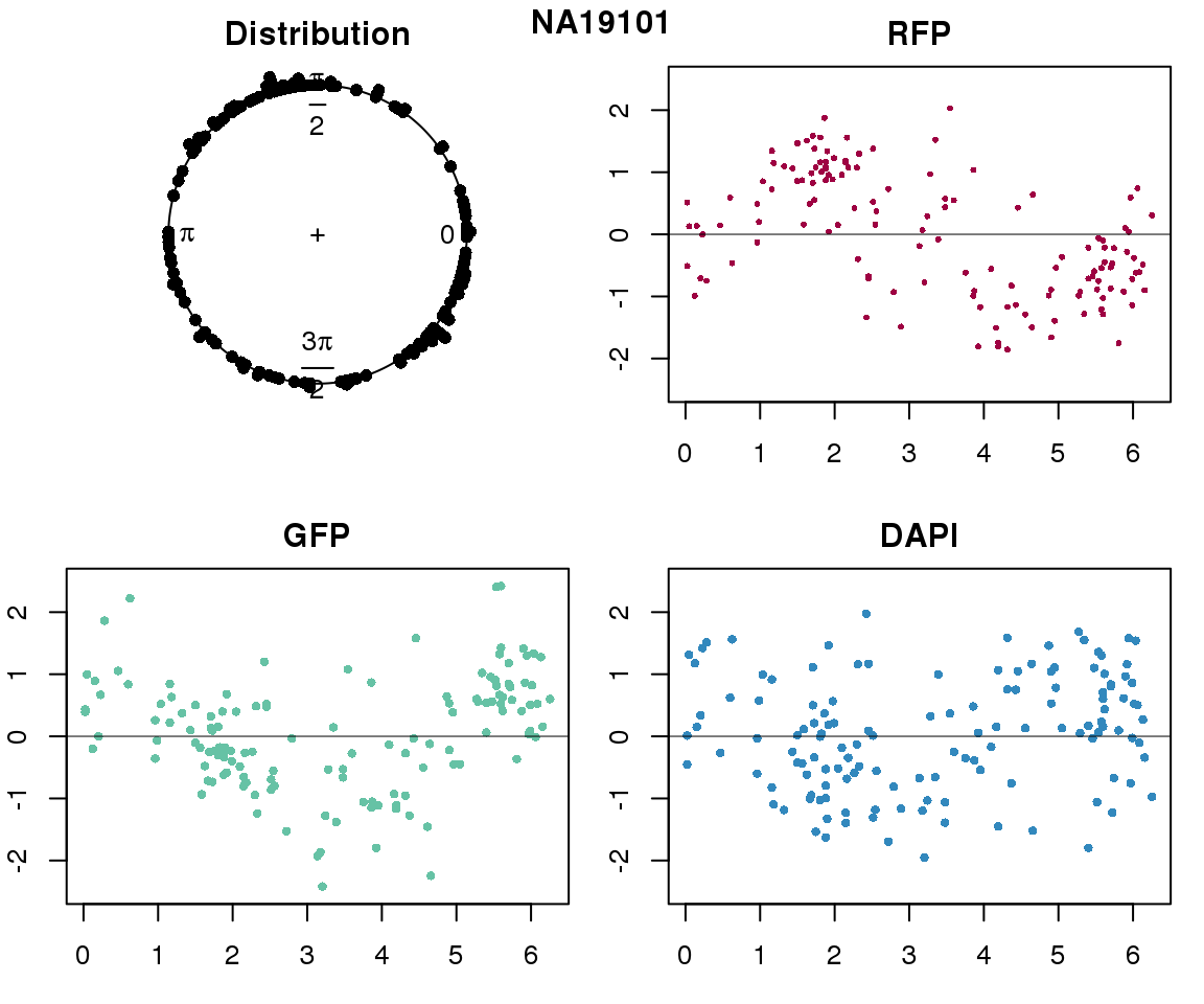
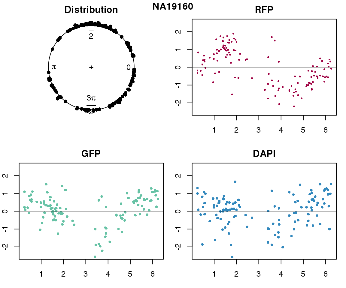
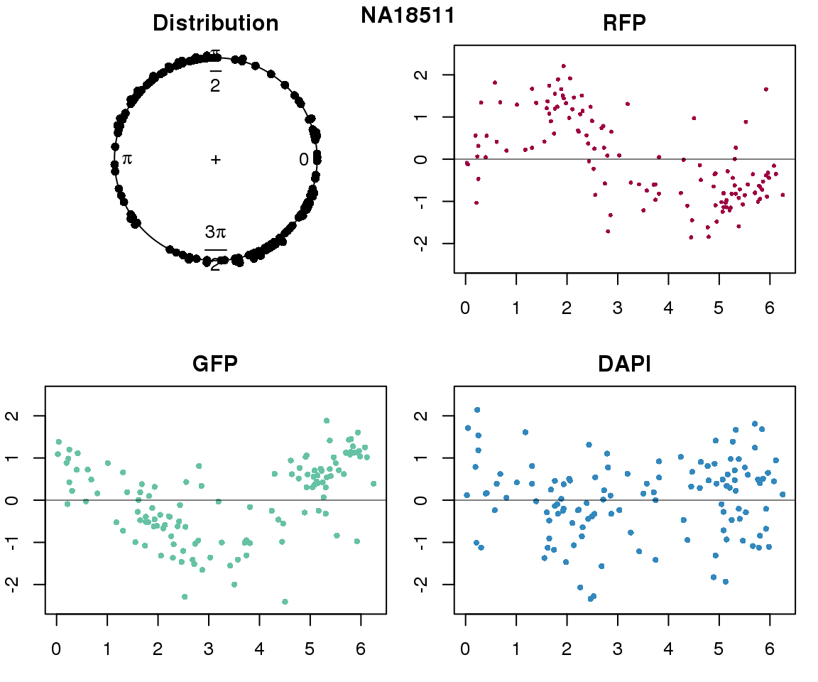
Property of the circle fit
Intensity values by circle fit
pdata.adj.filtered <- readRDS("../output/images-circle-ordering.Rmd/pdata.adj.filt.rds")
proj.res <- readRDS("../output/images-circle-ordering.Rmd/proj.res.rds")

for (i in 1:length(unique(pdata.adj.filt$chip_id))) {
  par(mfrow=c(2,2), mar = c(3,2,2,1))
  ids <- unique(as.character(pdata.adj.filt$chip_id))
  p_sub <- subset(pdata.adj.filt, chip_id == ids[i])
  #all.equal(rownames(p_sub), rownames(proj.res$NA18870[[1]]))
  plot(proj.res[[i]][[1]]$rads, stack=T, bins=180, main = "Distribution")
  library(RColorBrewer)
  color <- colorRampPalette(brewer.pal(11,"Spectral"))(11)
  plot(x=as.numeric(proj.res[[i]][[1]]$rads),
       y=p_sub$rfp.z, pch=16, cex=.5, col=color[1], ylim=c(-2.5, 2.5),
       xlab = "Position on the circle",
       ylab = "RFP", main = "RFP")
  abline(h=0, lwd=.5)
  plot(x=as.numeric(proj.res[[i]][[1]]$rads),
       y=p_sub$gfp.z, pch=16, cex=.7, col=color[9], ylim=c(-2.5, 2.5),
       xlab = "Position on the circle",
       ylab = "GFP", main = "GFP")
  abline(h=0, lwd=.5)
  plot(x=as.numeric(proj.res[[i]][[1]]$rads),
       y=p_sub$dapi.z, pch=16, cex=.7, col=color[10], ylim=c(-2.5, 2.5),
       xlab = "Position on the circle",
       ylab = "DAPI", main = "DAPI")
  abline(h=0, lwd=.5)
  title(names(proj.res)[i], outer=TRUE, line =-1)
}
Expression variation by cell time
# load cell cycle genes
genes.cycle <- readRDS("../output/seqdata-select-cellcyclegenes.Rmd/genes.cycle.detect.rds")

# log2cpm
log2cpm <- readRDS("../output/seqdata-batch-correction.Rmd/log2cpm.rds")
log2cpm.adjust <- readRDS("../output/seqdata-batch-correction.Rmd/log2cpm.adjust.rds")

counts.cycle <- counts[rownames(counts) %in% genes.cycle, ]
log2cpm.cycle <- log2cpm[rownames(log2cpm) %in% genes.cycle, ]
log2cpm.adjust.cycle <- log2cpm.adjust[rownames(log2cpm.adjust) %in% genes.cycle, ]
Pearson correlation
corrs <- lapply(1:length(unique(pdata.adj.filt$chip_id)), function(i) {

  id <- unique(pdata.adj.filt$chip_id)[i]

  log2cpm_sub <- log2cpm.adjust.cycle[, match(rownames(proj.res[[i]][[1]]), colnames(log2cpm.adjust.cycle))]

  counts_sub <- counts.cycle[, match(rownames(proj.res[[i]][[1]]), colnames(counts.cycle))]

  corrs <- do.call(rbind, lapply(1:nrow(counts_sub), function(g) {
    vec <- cbind(as.numeric(proj.res[[i]][[1]]$rads),
                 log2cpm_sub[g,])
    filt <- counts_sub[g,] > 1
    nsamp <- sum(filt)

    if (nsamp > ncol(counts_sub)/2) {
      vec <- vec[filt,]
      corr <- cor(vec[,1], vec[,2])
      nsam <- nrow(vec)
      data.frame(corr=corr, nsam=nsam)
    } else {
      data.frame(corr=NA, nsam=nrow(vec))
    }
    }))
  rownames(corrs) <- rownames(counts_sub)
  return(corrs)
  })
names(corrs) <- unique(pdata.adj.filt$chip_id)
par(mfrow=c(2,3))
for (i in 1:length(corrs)) {
hist(corrs[[i]]$corr, main = names(corrs)[i])
}
title(main = "Pearson correlation", outer = TRUE, line = -1)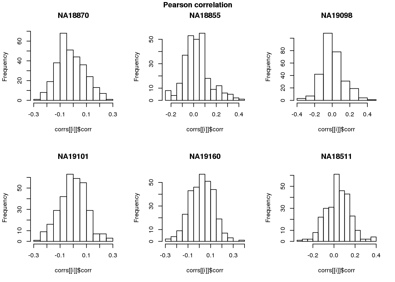
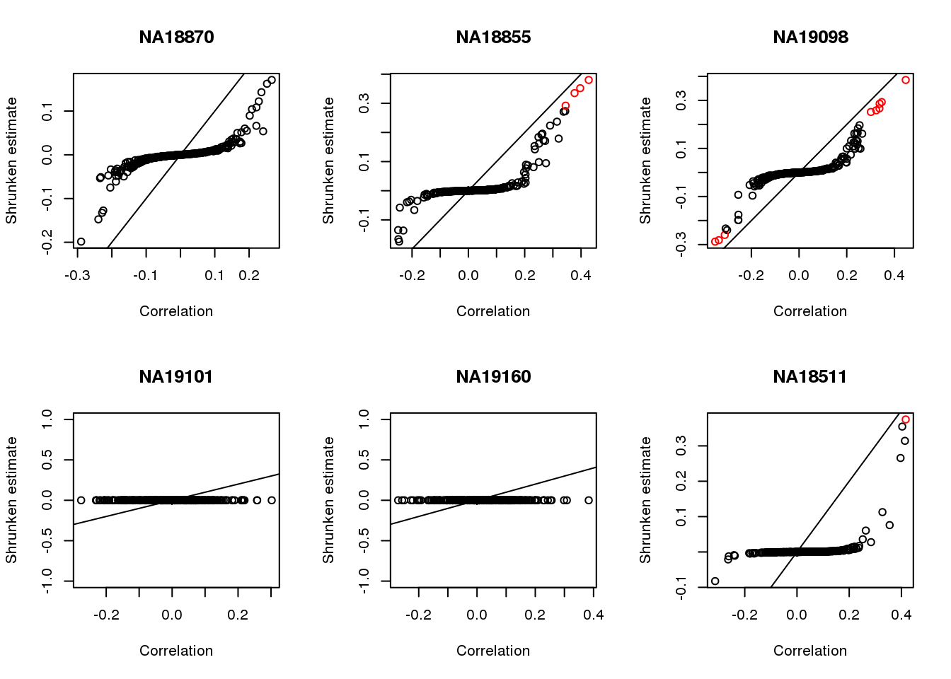
Apply CorShrink
par(mfrow=c(2,3))
for (i in 1:length(corrs)) {
  corrs_sub <- corrs[[i]]
  corr.shrink <- CorShrinkVector(corrs_sub$corr, nsamp_vec = corrs_sub$nsam,
                                   optmethod = "mixEM", report_model = TRUE)
  names(corr.shrink$estimate) <- rownames(corrs_sub)
  plot(corr.shrink$model$result$betahat,
       corr.shrink$model$result$PosteriorMean,
       col = 1+as.numeric(corr.shrink$model$result$svalue < .01),
       xlab = "Correlation", ylab = "Shrunken estimate")
  abline(0,1)
  title(names(corrs)[i])
}
Ciruclar correlation
source("../code/corr.cl.R")

corrs.cl <- lapply(1:length(unique(pdata.adj.filt$chip_id)), function(i) {

  id <- unique(pdata.adj.filt$chip_id)[i]

  log2cpm_sub <- log2cpm.adjust.cycle[, match(rownames(proj.res[[i]][[1]]), colnames(log2cpm.adjust.cycle))]

  counts_sub <- counts.cycle[, match(rownames(proj.res[[i]][[1]]), colnames(counts.cycle))]

  corrs <- do.call(rbind, lapply(1:nrow(counts_sub), function(g) {
    vec <- cbind(as.numeric(proj.res[[i]][[1]]$rads),
                 log2cpm_sub[g,])
    filt <- counts_sub[g,] > 1
    nsamp <- sum(filt)

    if (nsamp > ncol(counts_sub)/2) {
      vec <- vec[filt,]
      corr <- R2xtCorrCoeff(lvar=vec[,2], cvar=vec[,1])
      nsam <- nrow(vec)
      data.frame(corr=corr, nsam=nsam)
    } else {
      data.frame(corr=NA, nsam=nrow(vec))
    }
    }))
  rownames(corrs) <- rownames(counts_sub)
  return(corrs)
  })
names(corrs.cl) <- unique(pdata.adj.filt$chip_id)
par(mfrow=c(2,3))
for (i in 1:length(corrs)) {
hist(corrs.cl[[i]]$corr, main = names(corrs)[i])
}
title(main = "Circular-linear correlation", outer = TRUE, line = -1)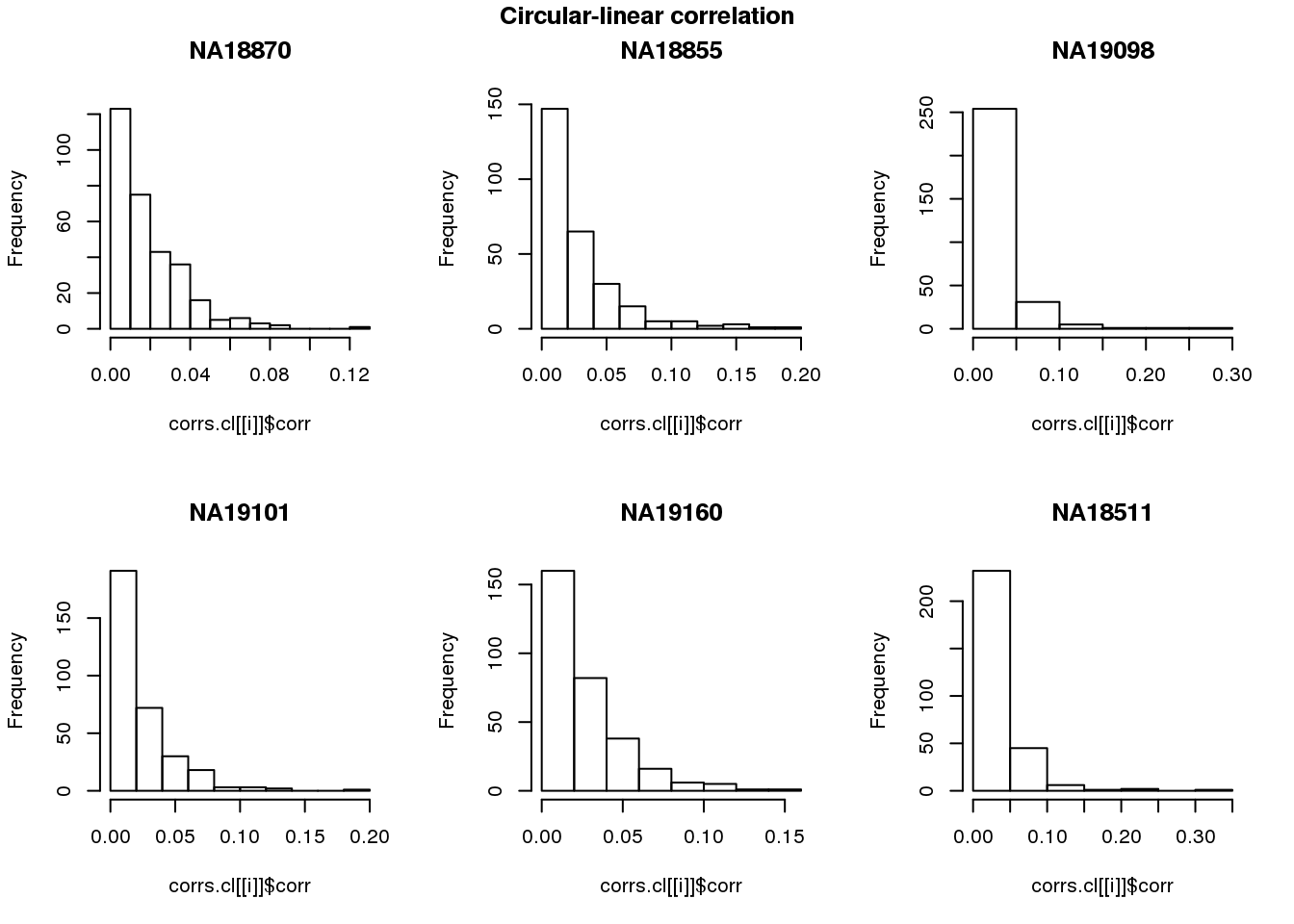
Compute significance value
corrs.cl.sig <- lapply(1:length(unique(pdata.adj.filt$chip_id)), function(i) {
id <- unique(pdata.adj.filt$chip_id)[i]
log2cpm_sub <- log2cpm.adjust.cycle[, match(rownames(proj.res[[i]][[1]]), colnames(log2cpm.adjust.cycle))]
counts_sub <- counts.cycle[, match(rownames(proj.res[[i]][[1]]), colnames(counts.cycle))]
corrs <- do.call(rbind, lapply(1:nrow(counts_sub), function(g) {
vec <- cbind(as.numeric(proj.res[[i]][[1]]$rads),
log2cpm_sub[g,])
filt <- counts_sub[g,] > 1
nsamp <- sum(filt)
if (nsamp > ncol(counts_sub)/2) {
vec <- vec[filt,]
corr <- R2xtIndTestRand(lvar=vec[,2], cvar=vec[,1], NR=100)
nsam <- nrow(vec)
return(corr)
} else {
return(data.frame(corr=NA, pval=NA))
}
}))
rownames(corrs) <- rownames(counts_sub)
return(corrs)
})
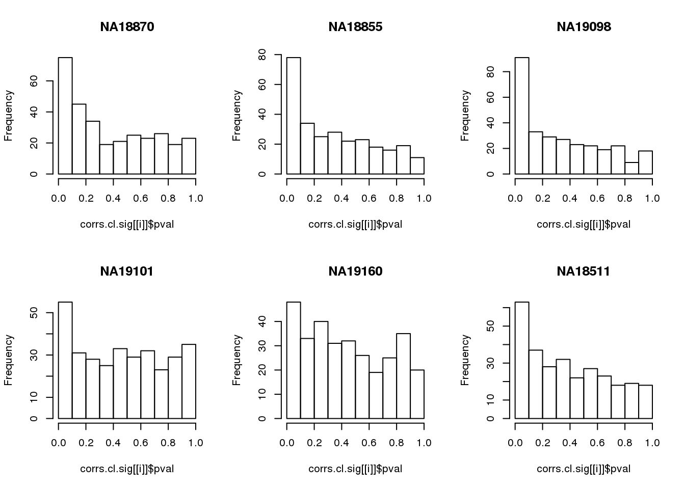
names(corrs.cl.sig) <- unique(pdata.adj.filt$chip_id)par(mfrow=c(2,3))
for(i in 1:length(corrs.cl.sig)) {
hist(corrs.cl.sig[[i]]$pval,
main = names(corrs.cl.sig)[i])
}
Consider significant ones
for (i in 1:length(corrs.cl.sig)) {
  ii.sig <- corrs.cl.sig[[i]]$pval < .01
  print(sum(ii.sig, na.rm=TRUE))
}
[1] 12
[1] 21
[1] 23
[1] 11
[1] 4
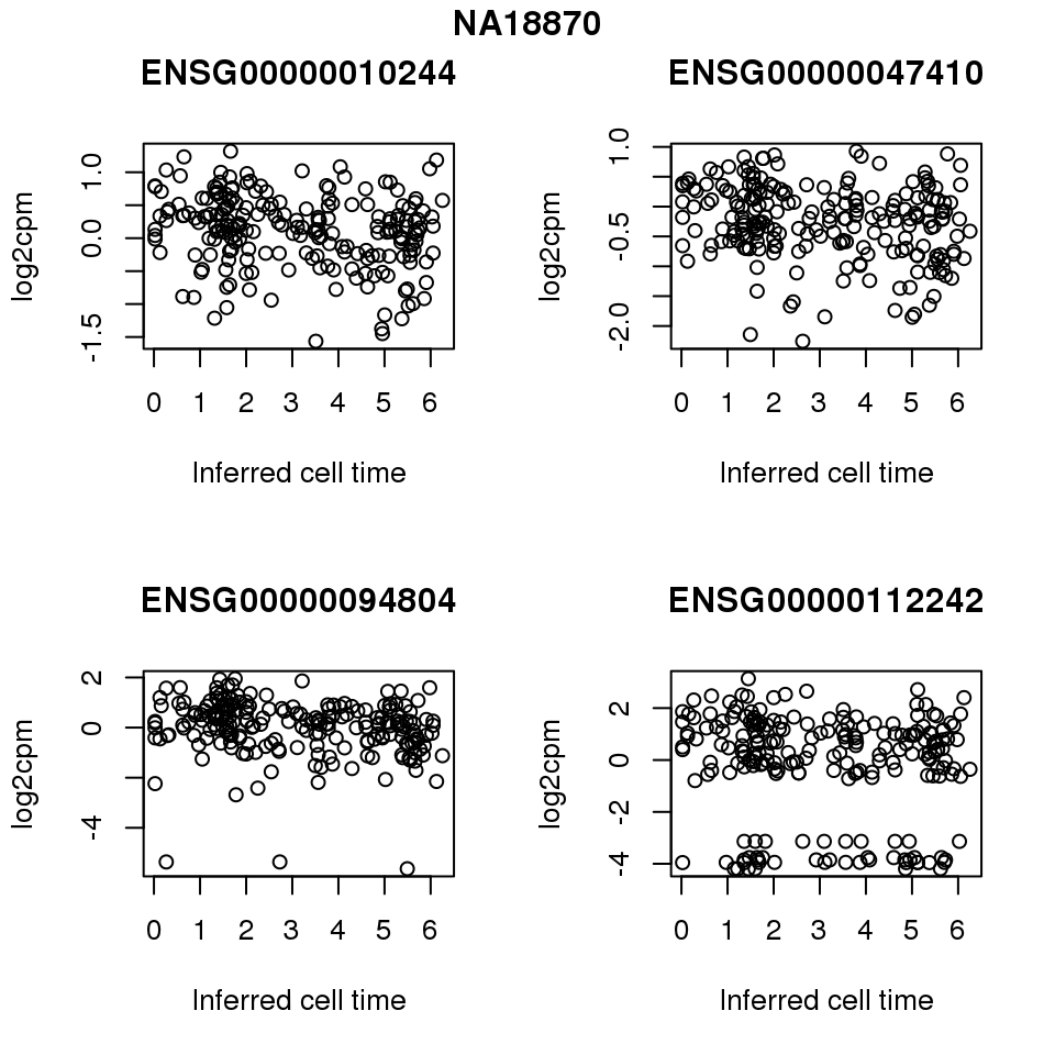
[1] 10Print some genes
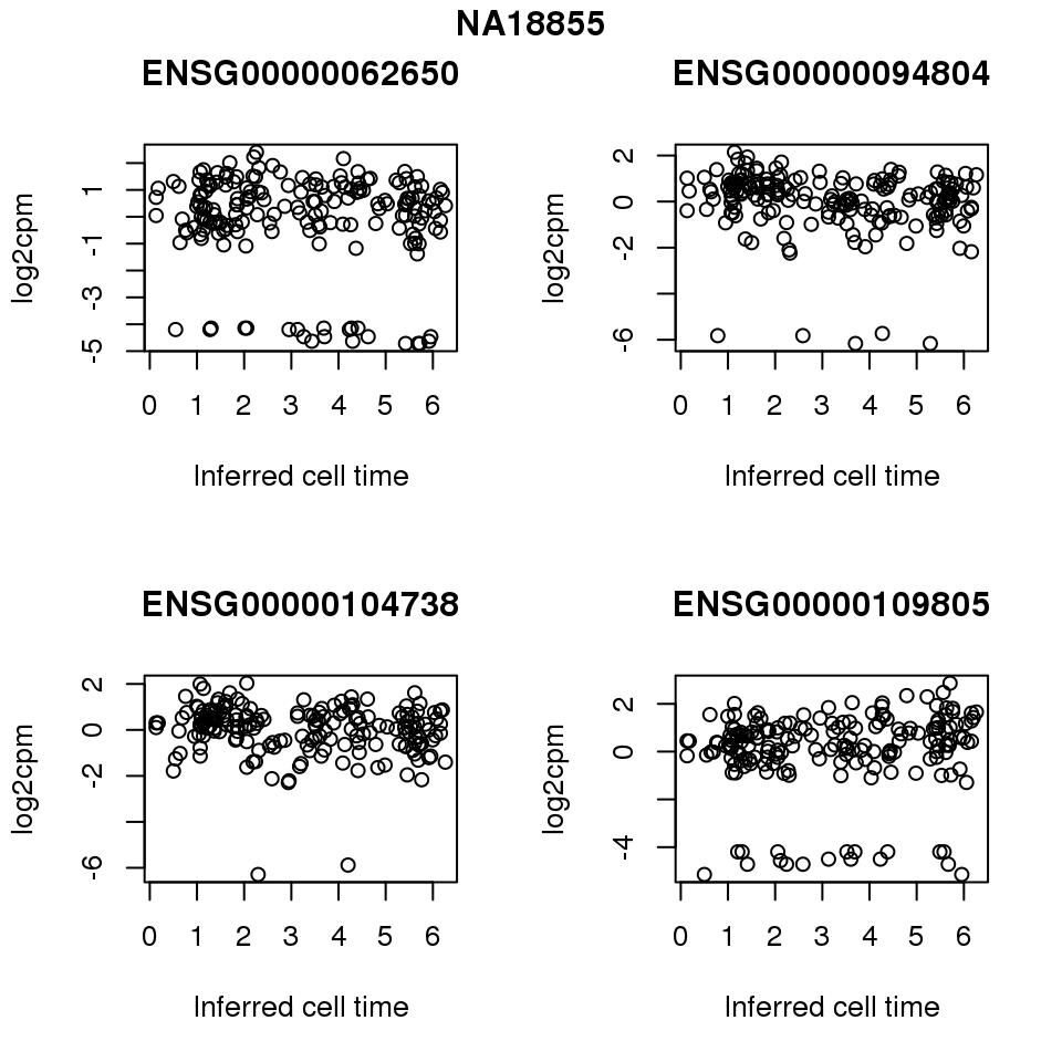
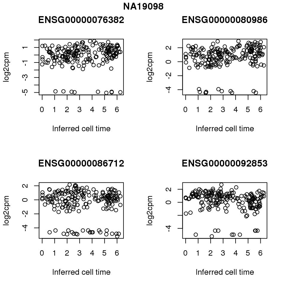
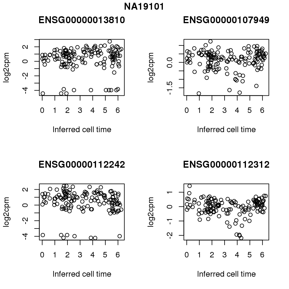
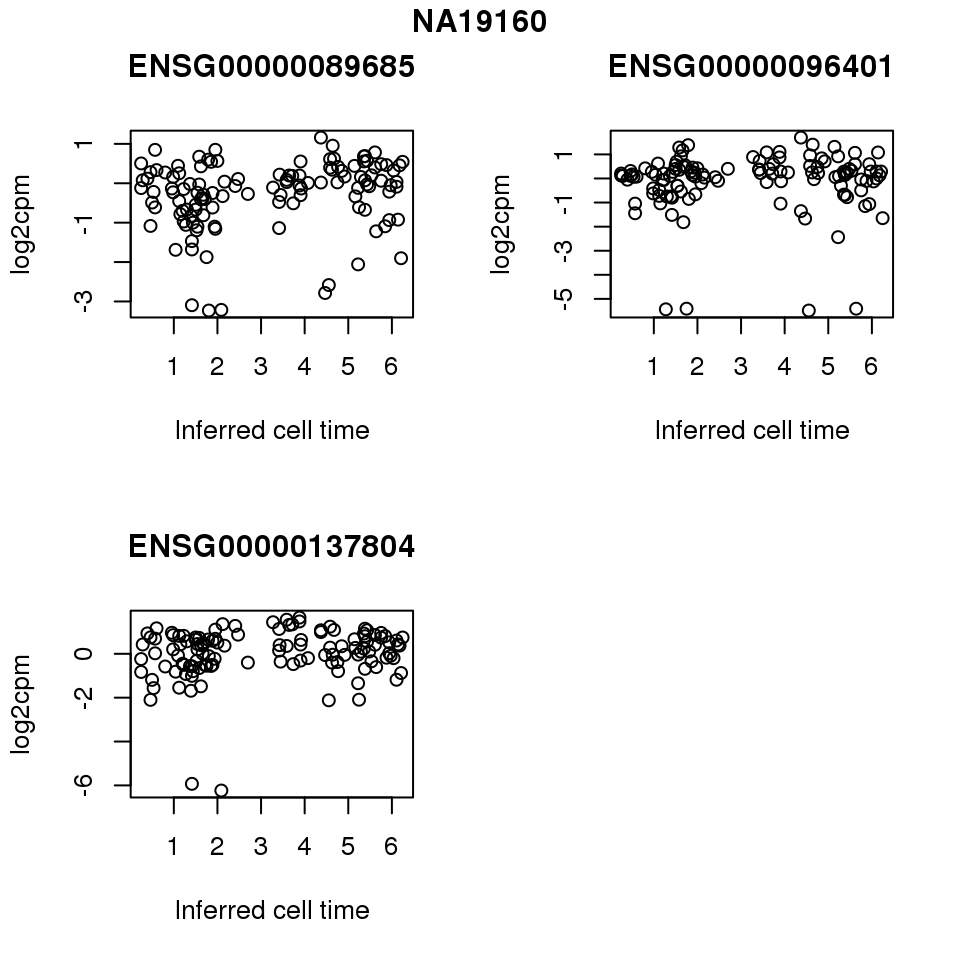
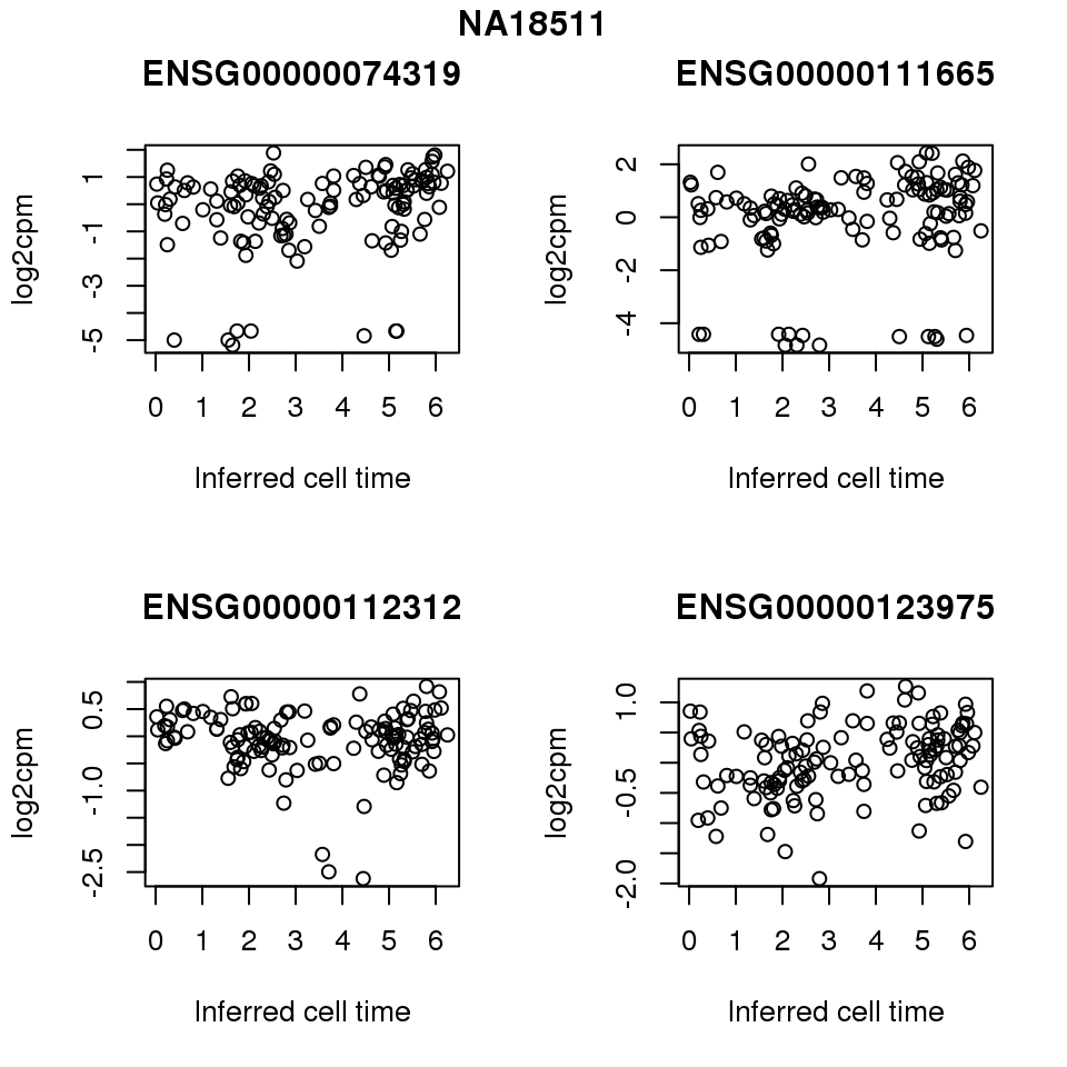
for (i in 1:length(corrs.cl.sig)) {
  ii.sig <- corrs.cl.sig[[i]]$pval < .01

  id <- unique(pdata.adj.filt$chip_id)[i]

  log2cpm_sub <- log2cpm.adjust.cycle[, match(rownames(proj.res[[i]][[1]]), colnames(log2cpm.adjust.cycle))]

  genes <- rownames(corrs.cl.sig[[i]])

  if (i == 5) {numgene <- 3} else {numgene <- 4}
  par(mfrow=c(2,2))
  for (g in 1:numgene) {
    gene <- genes[which(ii.sig)[g]]
    plot(x=as.numeric(proj.res[[i]][[1]]$rads),
         y = log2cpm_sub[rownames(log2cpm_sub) == gene,] ,
         xlab = "Inferred cell time",
         ylab = "log2cpm",
         main = gene)
  }
  title(names(proj.res)[i], outer = TRUE, line = -1)
}
Session information
R version 3.4.1 (2017-06-30)
Platform: x86_64-redhat-linux-gnu (64-bit)
Running under: Scientific Linux 7.2 (Nitrogen)

Matrix products: default
BLAS/LAPACK: /usr/lib64/R/lib/libRblas.so

locale:
 [1] LC_CTYPE=en_US.UTF-8       LC_NUMERIC=C
 [3] LC_TIME=en_US.UTF-8        LC_COLLATE=en_US.UTF-8
 [5] LC_MONETARY=en_US.UTF-8    LC_MESSAGES=en_US.UTF-8
 [7] LC_PAPER=en_US.UTF-8       LC_NAME=C
 [9] LC_ADDRESS=C               LC_TELEPHONE=C
[11] LC_MEASUREMENT=en_US.UTF-8 LC_IDENTIFICATION=C

attached base packages:
[1] parallel  stats     graphics  grDevices utils     datasets  methods
[8] base

other attached packages:
 [1] RColorBrewer_1.1-2  bindrcpp_0.2        CorShrink_0.1.1
 [4] matrixStats_0.53.1  dplyr_0.7.4         Biobase_2.38.0
 [7] BiocGenerics_0.24.0 conicfit_1.0.4      geigen_2.1
[10] pracma_2.1.4        circular_0.4-93

loaded via a namespace (and not attached):
 [1] Rcpp_0.12.15      plyr_1.8.4        compiler_3.4.1
 [4] pillar_1.1.0      git2r_0.21.0      bindr_0.1
 [7] iterators_1.0.9   tools_3.4.1       boot_1.3-19
[10] digest_0.6.15     evaluate_0.10.1   tibble_1.4.2
[13] lattice_0.20-35   pkgconfig_2.0.1   rlang_0.2.0
[16] foreach_1.4.4     Matrix_1.2-10     yaml_2.1.16
[19] mvtnorm_1.0-7     stringr_1.3.0     knitr_1.20
[22] rprojroot_1.3-2   grid_3.4.1        glue_1.2.0
[25] R6_2.2.2          rmarkdown_1.8     reshape2_1.4.3
[28] ashr_2.2-4        magrittr_1.5      MASS_7.3-47
[31] codetools_0.2-15  backports_1.1.2   htmltools_0.3.6
[34] assertthat_0.2.0  stringi_1.1.6     pscl_1.5.2
[37] doParallel_1.0.11 truncnorm_1.0-7   SQUAREM_2017.10-1
This R Markdown site was created with workflowr