Expression profile of the gold-standard samples
Joyce Hsiao
Last updated: 2018-02-26
Code version: 3206926
Overview/Results
Goal: Assess the expression profiles associated with cell cycle phase labels in a subset of samples identified to have high signal in intensity data (see here for details on how we selected the samples).
Method:
* Compute phase-specific score for within clusters and individuals. This method was previously used in [Macosko et al. 2015](http://dx.doi.org/10.1016/j.cell.2015.05.002) for identifying gene expression patterns that varied along cell cycle phases, and for summarizing cell cycle phase profile for single cell samples.
* We applied the 544 genes identified as varied in [Macosko et al. 2015](http://dx.doi.org/10.1016/j.cell.2015.05.002) and identified ~230 genes within individuals that varied in expression patterns.
* The method was applied to log2CPM normalized data. Briefly,
1. Identify the variable genes wihtin each cell cycle phase: compute for each cell-cycle phase, correlation between per-gene expression level and mean gene expression levels across all single cell samples. Select genes with correlation > .3.
2. Compute phase-specific score: compute average expression across genes for each single cell samples.
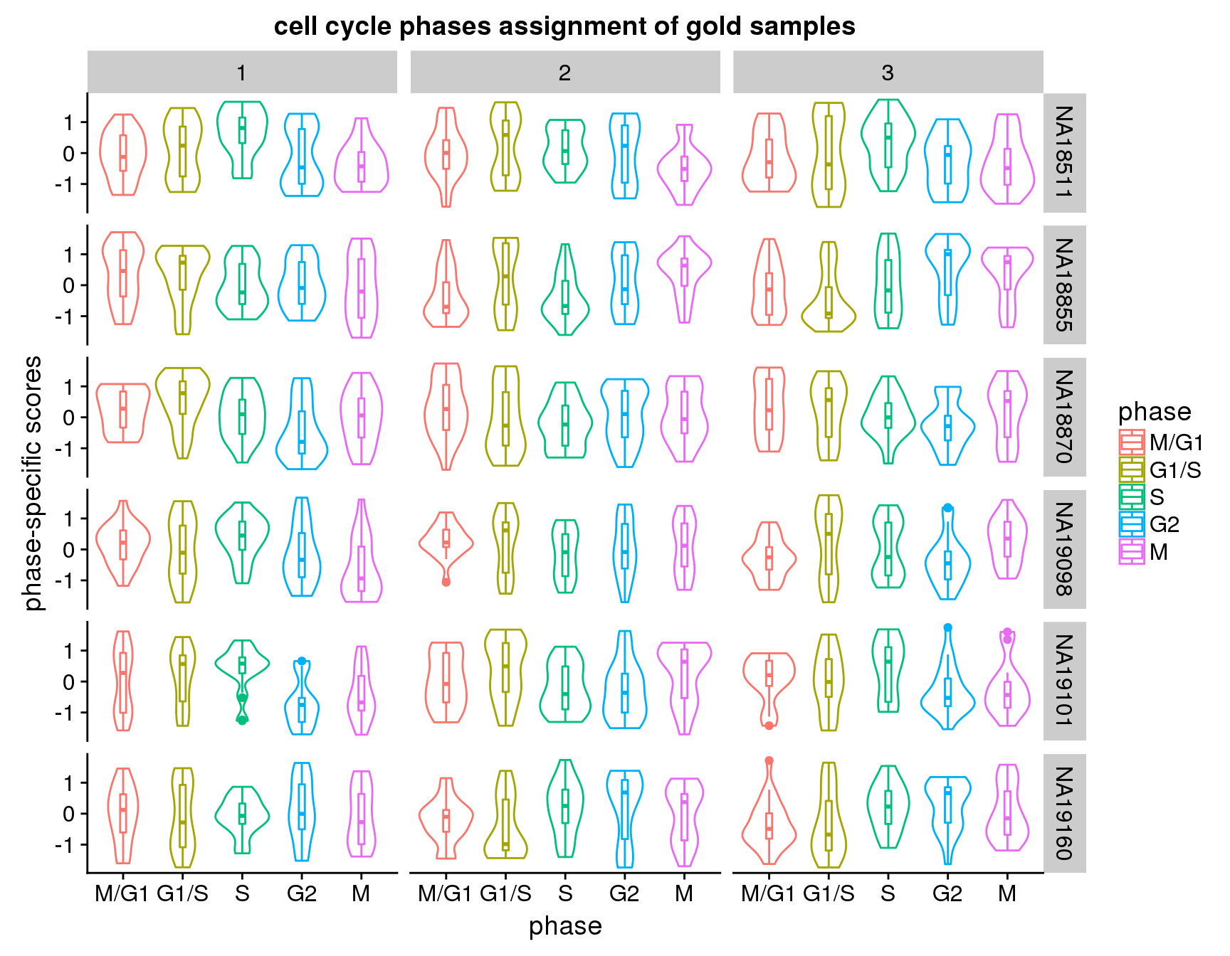
3. Standardize phase-specific scores in two-steps: within each phase, standardize (transforming to z-scores) scores across single cell samples, and then within each single cell sample, standardize scores across phase. Results:
* Within individaul analysis show that in genearl, cluster 2 and cluster 2 correspond to S and G2 phases as expected. Hoewver, cluster 1 cells do not correspond all to G1 phase as we hoped, and many cells score high on S phase. This is not as surprising as iPSC cell lines are known to have a short G1 phase. In our data, prior to C1 loading, we found only 5% of the samples that are possibly G1 phase (out of tens of thousands of cells).

* The genes used for the analysis were previously identified as "variable" or "cell cycle regulating" genes in [Macosko et al. 2015](http://dx.doi.org/10.1016/j.cell.2015.05.002). Applying the 544 genes in their results, we found 200 to 300 genes identified as "variable" in expression profiles along cell cycle phases. (NA18855 219 cells, NA18870 198 cells, NA19098 165 cells, NA19101 255 cells, NA19160 314 cells, NA18511 239 cells)

* For validity of the phase scores, we further apply the same method to data in [Leng et al. 2015](doi:10.1038/nmeth.3549), which have been previously scored for cell cycle phases also using FUCCI measurse. In that data, using the same set of genes, we found that these sorted cells score high in their corresponding phases.
Data and packages
Packages
library(Biobase)
library(ggplot2)
library(cowplot)
library(data.table)
library(tidyr)
library(gplots)
library(ccRemover)
Load data
df <- readRDS(file="../data/eset-filtered.rds")
pdata <- pData(df)
fdata <- fData(df)

# select endogeneous genes
counts <- exprs(df)[grep("ERCC", rownames(df), invert=TRUE), ]

# cpm normalization
log2cpm <- log2(t(t(counts+1)*(10^6)/colSums(counts)))
subset to include genes that are annotated as cell cycle genes (according to ccRemover)
ccremover <- readRDS("../data/cellcycle-genes-previous-studies/rds/macosko-2015.rds")
which_ccremover <- gene_indexer(rownames(log2cpm), species="human", name_type="symbol")

log2cpm_ccremover <- log2cpm[which_ccremover, ]
subset to include genes in Macosko data
macosko <- readRDS("../data/cellcycle-genes-previous-studies/rds/macosko-2015.rds")
which_macosko <- which(rownames(log2cpm) %in% macosko$ensembl)

log2cpm_macosko <- log2cpm[which_macosko, ]
ccgenes_macosko <- macosko[which(macosko$ensembl %in% rownames(log2cpm_macosko)),]
Load best subset. si_pam.rda contains two objects: si_pam_25 (top 25 samples within clusters and individuals) and si_pam_long (all sample information on silhouette index).
load(file = "../output/images-subset-silhouette.Rmd/si_pam.ash.rda")subset to the best samples
log2cpm_macosko_top <- log2cpm_macosko[, rownames(pdata) %in% unique(si_pam_25$unique_id)]
pdata_top <- pdata[rownames(pdata) %in% unique(si_pam_25$unique_id),]
all.equal(colnames(log2cpm_macosko_top), rownames(pdata_top))
[1] TRUEWithin individuals assignment
chip_ids <- unique(pdata_top$chip_id)
all.equal(rownames(pdata_top), colnames(log2cpm_macosko_top))
[1] TRUEcc_scores_within <- lapply(1:uniqueN(pdata_top$chip_id), function(j) {
id <- chip_ids[j]
samples_to_select <- rownames(pdata_top)[which(pdata_top$chip_id == id)]
cc_scores_list <- lapply(1:uniqueN(ccgenes_macosko$phase), function(i) {
ph <- unique(ccgenes_macosko$phase)[i]
df_sub <- log2cpm_macosko_top[rownames(log2cpm_macosko_top) %in% ccgenes_macosko$ensembl[ccgenes_macosko$phase == ph], samples_to_select]
mn <- colMeans(df_sub)
cc <- cor(t(rbind(mn, df_sub)))
cc_mean <- cc[-1,1]
genes_cc <- names(cc_mean)[which(cc_mean > .3)]
scores_raw <- colMeans(df_sub[rownames(df_sub) %in% genes_cc,])
scores_z <- scale(scores_raw)
return(list(scores_z=scores_z, ngenes =length(genes_cc)))
})
names(cc_scores_list) <- unique(ccgenes_macosko$phase)
return(cc_scores_list)
})
names(cc_scores_within) <- chip_ids
ngenes_within <- lapply(cc_scores_within, function(x) {
sapply(x, function(y) y[[2]])
})
ngenes <- sapply(ngenes_within, function(x) sum(x))
print(ngenes)NA18855 NA18870 NA19098 NA19101 NA19160 NA18511
218 165 175 257 314 238 # compute phase-specific score for each gene set
cc_scores <- lapply(cc_scores_within, function(x) {
tmp <- do.call(cbind, lapply(x, "[[", 1))
colnames(tmp) <- unique(ccgenes_macosko$phase)
return(tmp)
})
# standardize scores across phases
cc_scores_z <- lapply(cc_scores, function(x) {
tmp <- t(apply(x, 1, scale))
colnames(tmp) <- unique(ccgenes_macosko$phase)
tmp <- as.data.frame(tmp)
return(tmp)
})
# convert data format from wide to long
cc_scores_z_long <- lapply(cc_scores_z, function(x) {
long <- gather(x, key=phase, value=scores)
long$uniqe_id <- rep(rownames(x), ncol(x))
long$chip_id <- pdata_top$chip_id[match(long$uniqe_id, rownames(pdata_top))]
long$experiment <- pdata_top$experiment[match(long$uniqe_id, rownames(pdata_top))]
# select gold standard set
long$cluster <- si_pam_25$cluster[match(long$uniqe_id, si_pam_25$unique_id)]
long$phase <- factor(long$phase, levels=c("M/G1", "G1/S", "S", "G2", "M"))
long$cluster <- as.factor(long$cluster)
return(long)
})
Across individuals assignment
cc_scores_list <- lapply(1:uniqueN(ccgenes_macosko$phase), function(i) {
  ph <- unique(ccgenes_macosko$phase)[i]
  df_sub <- log2cpm_macosko_top[rownames(log2cpm_macosko_top) %in% ccgenes_macosko$ensembl[ccgenes_macosko$phase == ph],]
  mn <- colMeans(df_sub)
  cc <- cor(t(rbind(mn, df_sub)))
  cc_mean <- cc[-1,1]
  genes_cc <- names(cc_mean)[which(cc_mean > .3)]
  scores_raw <- colMeans(df_sub[rownames(df_sub) %in% genes_cc,])
  scores_z <- scale(scores_raw)
  return(list(scores_z=scores_z, ngenes =length(genes_cc)))
})
names(cc_scores_list) <- unique(ccgenes_macosko$phase)

ngenes <- sapply(cc_scores_list, "[[", 2)
cc_scores <- do.call(cbind, lapply(cc_scores_list, "[[", 1))
colnames(cc_scores) <- unique(ccgenes_macosko$phase)

# standardize scores across phases
cc_scores_z <- t(apply(cc_scores, 1, scale))
colnames(cc_scores_z) <- unique(ccgenes_macosko$phase)
cc_scores_z <- as.data.frame(cc_scores_z)

# convert data format from wide to long
cc_scores_z_long <- gather(cc_scores_z, key=phase, value=cc_scores_z)
cc_scores_z_long$uniqe_id <- rep(rownames(cc_scores_z), ncol(cc_scores_z))

cc_scores_z_long$chip_id <- pdata$chip_id[match(cc_scores_z_long$uniqe_id, rownames(pdata))]
cc_scores_z_long$experiment <- pdata$experiment[match(cc_scores_z_long$uniqe_id, rownames(pdata))]

# select gold standard set
cc_scores_z_long$cluster <- si_pam_25$cluster[match(cc_scores_z_long$uniqe_id, si_pam_25$unique_id)]

cc_scores_z_long$phase <- factor(cc_scores_z_long$phase,
                                  levels=c("M/G1", "G1/S", "S", "G2", "M"))
cc_scores_z_long$cluster <- as.factor(cc_scores_z_long$cluster)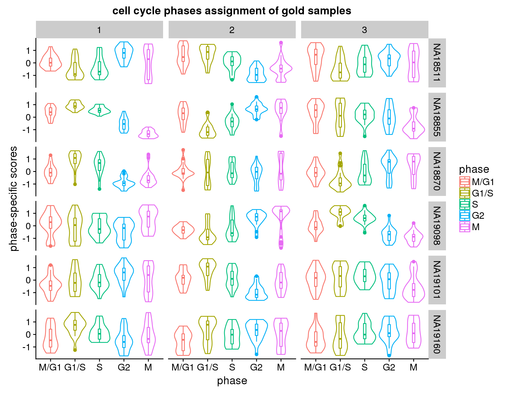
Others
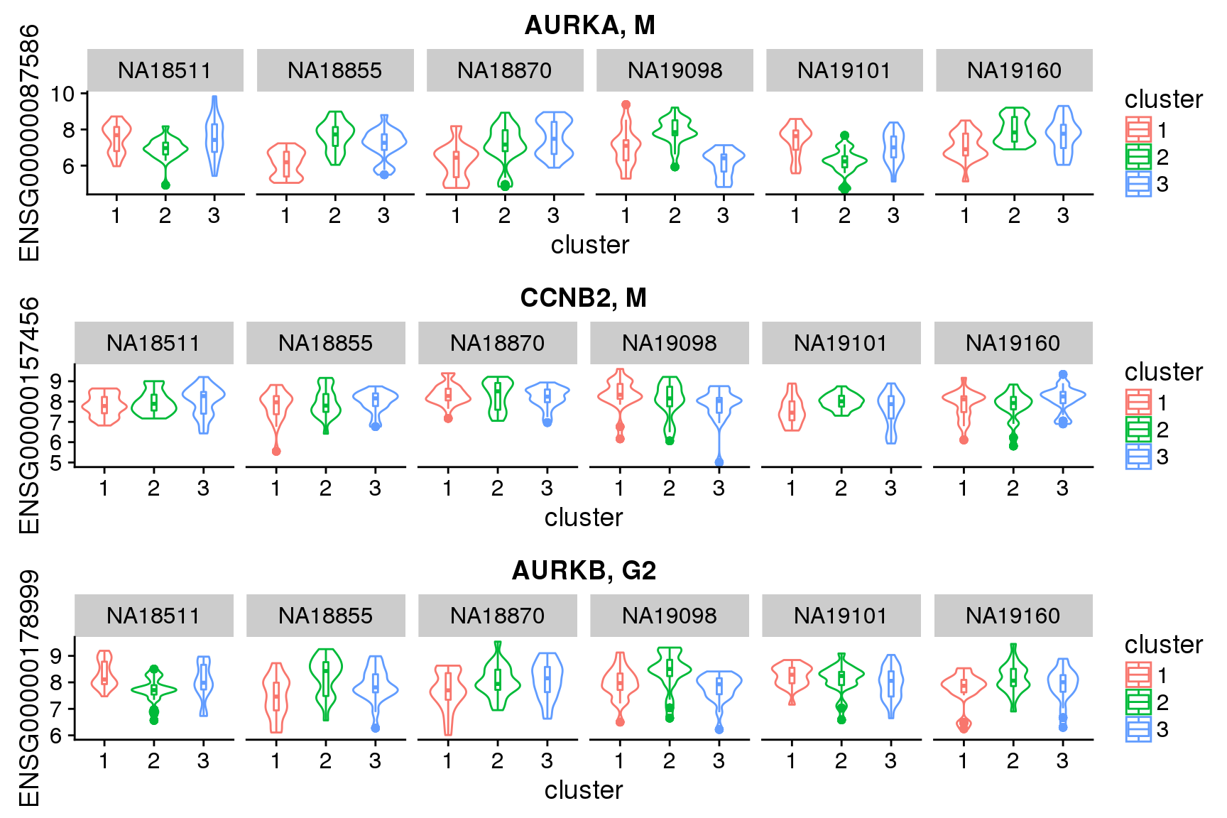
Look up “classical cell cycle genes” listed in Macosko et al. 2015 and see their patterns across the assigned clusters.
hgnc <- c("CCNB1", "CCNB2", "MCM2", "MCM3", "MCM4", "MCM5", "MCM6",
          "MCM7", "MCM10", "AURKA", "AURKB")
ensg <- ccgenes_macosko$ensembl[which(ccgenes_macosko$hgnc %in% hgnc)]
tmp <- log2cpm_macosko[which(rownames(log2cpm_macosko) %in% ensg),]
tmp <- data.frame(t(tmp))

cc_scores_z_long$ENSG00000073111 <- tmp$ENSG00000073111[match(cc_scores_z_long$uniqe_id, rownames(tmp))]
cc_scores_z_long$ENSG00000076003 <- tmp$ENSG00000076003[match(cc_scores_z_long$uniqe_id, rownames(tmp))]
cc_scores_z_long$ENSG00000087586 <- tmp$ENSG00000087586[match(cc_scores_z_long$uniqe_id, rownames(tmp))]
cc_scores_z_long$ENSG00000076003 <- tmp$ENSG00000076003[match(cc_scores_z_long$uniqe_id, rownames(tmp))]
cc_scores_z_long$ENSG00000100297 <- tmp$ENSG00000100297[match(cc_scores_z_long$uniqe_id, rownames(tmp))]
cc_scores_z_long$ENSG00000157456 <- tmp$ENSG00000157456[match(cc_scores_z_long$uniqe_id, rownames(tmp))]
cc_scores_z_long$ENSG00000178999 <- tmp$ENSG00000178999[match(cc_scores_z_long$uniqe_id, rownames(tmp))]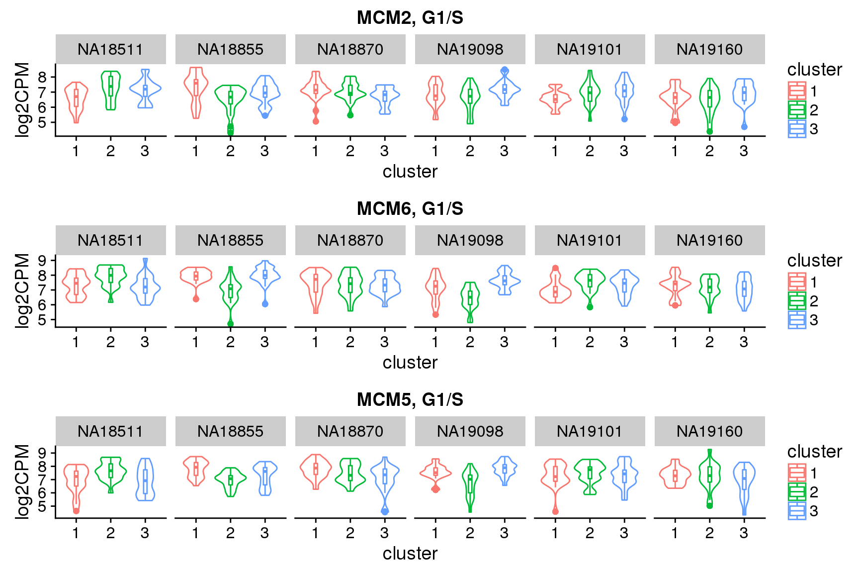
Session information
R version 3.4.1 (2017-06-30)
Platform: x86_64-redhat-linux-gnu (64-bit)
Running under: Scientific Linux 7.2 (Nitrogen)

Matrix products: default
BLAS/LAPACK: /usr/lib64/R/lib/libRblas.so

locale:
 [1] LC_CTYPE=en_US.UTF-8       LC_NUMERIC=C
 [3] LC_TIME=en_US.UTF-8        LC_COLLATE=en_US.UTF-8
 [5] LC_MONETARY=en_US.UTF-8    LC_MESSAGES=en_US.UTF-8
 [7] LC_PAPER=en_US.UTF-8       LC_NAME=C
 [9] LC_ADDRESS=C               LC_TELEPHONE=C
[11] LC_MEASUREMENT=en_US.UTF-8 LC_IDENTIFICATION=C

attached base packages:
[1] parallel  stats     graphics  grDevices utils     datasets  methods
[8] base

other attached packages:
[1] ccRemover_1.0.4     gplots_3.0.1        tidyr_0.8.0
[4] data.table_1.10.4-3 cowplot_0.9.2       ggplot2_2.2.1
[7] Biobase_2.38.0      BiocGenerics_0.24.0

loaded via a namespace (and not attached):
 [1] Rcpp_0.12.15       pillar_1.1.0       compiler_3.4.1
 [4] git2r_0.21.0       plyr_1.8.4         bitops_1.0-6
 [7] tools_3.4.1        digest_0.6.15      evaluate_0.10.1
[10] tibble_1.4.2       gtable_0.2.0       rlang_0.2.0
[13] yaml_2.1.16        stringr_1.3.0      knitr_1.20
[16] gtools_3.5.0       caTools_1.17.1     rprojroot_1.3-2
[19] grid_3.4.1         glue_1.2.0         rmarkdown_1.8
[22] gdata_2.18.0       purrr_0.2.4        reshape2_1.4.3
[25] magrittr_1.5       backports_1.1.2    scales_0.5.0
[28] htmltools_0.3.6    colorspace_1.3-2   labeling_0.3
[31] KernSmooth_2.23-15 stringi_1.1.6      lazyeval_0.2.1
[34] munsell_0.4.3
This R Markdown site was created with workflowr