Classify cells based on FUCCI using mixture modeling
Joyce Hsiao
Last updated: 2018-01-26
Code version: 6aa2392
Overview/Results
I tried normal-based mixture modeling on the data that have already been filtered for quality single cells using both RNA-sequencing and microscopy data. The eventual goal is to select a subset of cells that are “representative” of each cell cycle phase.
I used Mclust package which fits mixtures of normal distributions with a variety of covariance structure. I allowed Mclust to fit all possible covariance structures and select the best-fit structure as the final result.
\(~\)
Results:
First, note that the 990 samples in this dataset passed microscopy filters and sequencing data filters. Microscopy filters based on DAPI intensities exlude samples that are detected with low or no DNA content and also samples with more than one nucleus. In other words, microscopy filters exclude cells that are in G0 phase, which typically have low DNA content. In addition, microscopy filters based on GFP and RFP exlude samples that are either in G0 phase or in M phase.
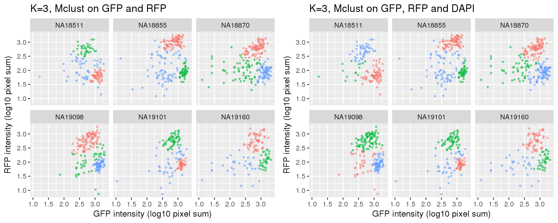
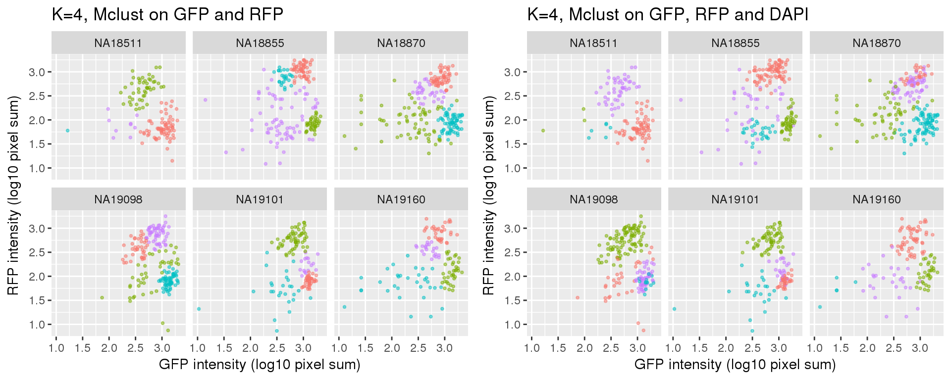
Standard flow cytometry analysis using GFP and RFP can classify cells into G1, G1/S, and G2/M. We fit k=3 and k=4 using PAM on GFP and RFP and also on GFP, RFP, and DAPI.
Results for either k=3 or k=4 didn’t change after adding DAPI measurements.
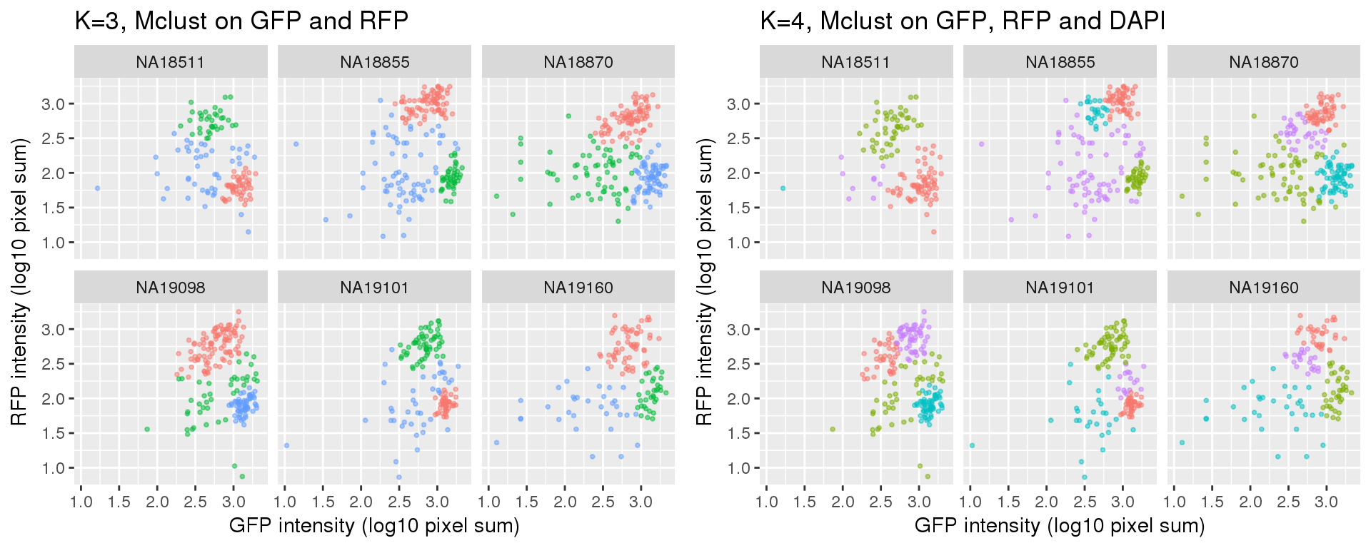
Results of partitions between k=3 and k=4: I am mainly interested in k=3 case. I will use k=4 results in the quality checks for k=3 results. In brief, I’ll look at cell cycle gene expression profiles of both of these cases. If the additional partition in k=4 is similar to one of the other three partitions, then we can say k=3 fits better.
After we decide on the clustering of cells, we can compute silhouette index for each cell to determine how well each cell fits into its cluster. Then, we can use silhouette index to choose the most “represented cells” from each cluster, for example selecting cells that are the closet to cluster centers.
Compared to the resutls using PAM. normal-based mixture modeling results are highly influenced by outliers, and the clusters can overlap in the density region of GFP by RFP. These results make the normal-based mixture modeling results undesirable for classifying cell cycle phase. However, it remains to be seen that which of these two methods provide a better set of representative cells of cell cycle phases.
Data and packages
Packages
library(Biobase)
library(ggplot2)
library(cowplot)
library(mclust)
library(data.table)
Load data
df <- readRDS(file="../data/eset-filtered.rds")
pdata <- pData(df)
fdata <- fData(df)

# select endogeneous genes
counts <- exprs(df)[grep("ERCC", rownames(df), invert=TRUE), ]

# cpm normalization
log2cpm <- log2(t(t(counts+1)*(10^6)/colSums(counts)))
select cell cycle genes
cellcycle <- readRDS("../data/cellcycle-genes-previous-studies/rds/macosko-2017.rds")
which_cc <- which(rownames(log2cpm) %in% cellcycle$ensembl)

log2cpm_cc <- log2cpm[which_cc, ]
Analysis
Fitting mclust for cells using only green and red intensity measurements.
ints <- with(pdata, data.frame(rfp.median.log10sum,
                               gfp.median.log10sum,
                               dapi.median.log10sum))
ints <- data.frame(ints,
                   chip_id = as.factor(pdata$chip_id))

k_list <- c(3:4)

fit_green_red <- lapply(k_list, function(k) {
  fit <- lapply(1:uniqueN(ints$chip_id), function(i) {
    df_sub <- subset(ints, chip_id==unique(chip_id)[i],
                     select = -c(chip_id, dapi.median.log10sum))
    fit_sub <- Mclust(df_sub, G=k)
    return(fit_sub)
  })
  names(fit) <- unique(ints$chip_id)
  return(fit)
})
names(fit_green_red) <- paste0("k", k_list)

fit_green_red_plot <- vector("list", length(fit_green_red))
for (k in c(1:length(k_list))) {
  pp <- do.call(rbind, lapply(1:uniqueN(ints$chip_id), function(i) {
    df_sub <- subset(ints, chip_id==unique(chip_id)[i])
    df_sub <- data.frame(df_sub, cluster=as.factor(fit_green_red[[k]][[i]]$classification))
    return(df_sub)
  }))
  fit_green_red_plot[[k]] <- pp
}
Fitting for cells using all three intensity measurements.
fit_green_red_dapi <- lapply(k_list, function(k) {
  fit <- lapply(1:uniqueN(ints$chip_id), function(i) {
    df_sub <- subset(ints, chip_id==unique(chip_id)[i],
                     select = -chip_id)
    fit_sub <- Mclust(df_sub, G=k)
    return(fit_sub)
  })
  names(fit) <- unique(ints$chip_id)
  return(fit)
})
names(fit_green_red_dapi) <- paste0("k", k_list)

fit_green_red_dapi_plot <- vector("list", length(fit_green_red_dapi))
for (k in c(1:length(k_list))) {
  pp <- do.call(rbind, lapply(1:uniqueN(ints$chip_id), function(i) {
    df_sub <- subset(ints, chip_id==unique(chip_id)[i])
    df_sub <- data.frame(df_sub, cluster=as.factor(fit_green_red_dapi[[k]][[i]]$classification))
    return(df_sub)
  }))
  fit_green_red_dapi_plot[[k]] <- pp
}
Results
k=3
k=4
k=3 versus k=4
Session information
R version 3.4.1 (2017-06-30)
Platform: x86_64-redhat-linux-gnu (64-bit)
Running under: Scientific Linux 7.2 (Nitrogen)

Matrix products: default
BLAS/LAPACK: /usr/lib64/R/lib/libRblas.so

locale:
 [1] LC_CTYPE=en_US.UTF-8       LC_NUMERIC=C
 [3] LC_TIME=en_US.UTF-8        LC_COLLATE=en_US.UTF-8
 [5] LC_MONETARY=en_US.UTF-8    LC_MESSAGES=en_US.UTF-8
 [7] LC_PAPER=en_US.UTF-8       LC_NAME=C
 [9] LC_ADDRESS=C               LC_TELEPHONE=C
[11] LC_MEASUREMENT=en_US.UTF-8 LC_IDENTIFICATION=C

attached base packages:
[1] parallel  stats     graphics  grDevices utils     datasets  methods
[8] base

other attached packages:
[1] data.table_1.10.4-3 mclust_5.4          cowplot_0.9.2
[4] ggplot2_2.2.1       Biobase_2.38.0      BiocGenerics_0.24.0

loaded via a namespace (and not attached):
 [1] Rcpp_0.12.14     knitr_1.17       magrittr_1.5     munsell_0.4.3
 [5] colorspace_1.3-2 rlang_0.1.4      stringr_1.2.0    plyr_1.8.4
 [9] tools_3.4.1      grid_3.4.1       gtable_0.2.0     git2r_0.20.0
[13] htmltools_0.3.6  yaml_2.1.16      lazyeval_0.2.1   rprojroot_1.3-1
[17] digest_0.6.13    tibble_1.3.4     evaluate_0.10.1  rmarkdown_1.8
[21] labeling_0.3     stringi_1.1.6    compiler_3.4.1   scales_0.5.0
[25] backports_1.1.2
This R Markdown site was created with workflowr