npreg: trendfilter

Data and packages

Packages

library(circular)
library(conicfit)
library(Biobase)
library(dplyr)
library(matrixStats)

library(genlasso)

Load data

df <- readRDS(file="../data/eset-final.rds")
pdata <- pData(df)
fdata <- fData(df)

# select endogeneous genes
counts <- exprs(df)[grep("ENSG", rownames(df)), ]

log2cpm.all <- t(log2(1+(10^6)*(t(counts)/pdata$molecules)))

macosko <- readRDS("../data/cellcycle-genes-previous-studies/rds/macosko-2015.rds")

theta <- readRDS("../output/images-time-eval.Rmd/theta.rds")
log2cpm.all.ord <- log2cpm.all[,order(theta)]

source("../code/utility.R")
source("../code/npreg/npreg.methods.R")

–

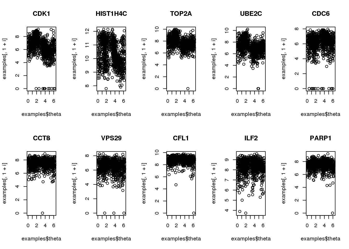
Consider 5 genes previously identified to be cyclical

Consider 5 genes previously identified to have cyclical patterns and 5 genes previously identified to not have cyclical patterns. Note that there’s a discrepany (albeit small) between the samples that was used to identify cyclical patterns and the samples that are in the finalized data.

examples <- readRDS("../output/npreg-methods.Rmd/cyclegenes.rds")

library(biomaRt)
ensembl <- useMart(biomart = "ensembl", dataset = "hsapiens_gene_ensembl")
symbols <- getBM(attributes = c("hgnc_symbol",'ensembl_gene_id'), 
      filters = c('ensembl_gene_id'),
      values = colnames(examples)[-1], 
      mart = ensembl)
symbols <- symbols[match(colnames(examples)[-1], symbols$ensembl_gene_id),]

par(mfrow=c(2,5))
for (i in 1:10) {
  plot(examples$theta,
       examples[,1+i], main = symbols$hgnc_symbol[i])
}

Get ENSG IDs.

cycles <- symbols[1:5,]
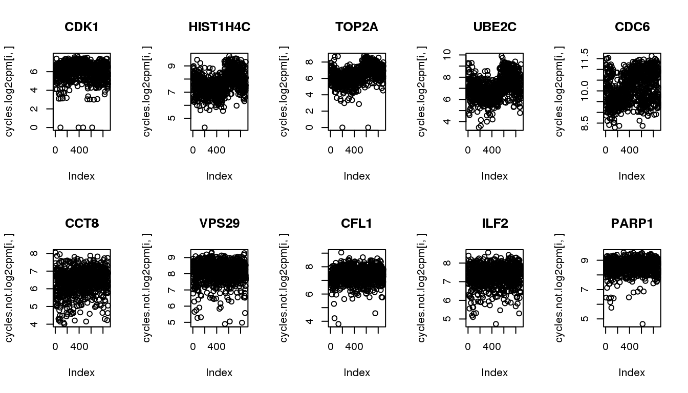
cycles.not <- symbols[6:10,]

Get these genes from the updated data.

cycles.log2cpm <- log2cpm.all.ord[rownames(log2cpm.all.ord) %in% cycles$ensembl_gene_id,]
cycles.not.log2cpm <- log2cpm.all.ord[rownames(log2cpm.all.ord) %in% cycles.not$ensembl_gene_id,]

confirm pattern in the udpated dataset.

par(mfrow=c(2,5))
for (i in 1:5) {
  plot(cycles.log2cpm[i,], main = cycles$hgnc_symbol[i])
}
for (i in 1:5) {
  plot(cycles.not.log2cpm[i,], main = cycles.not$hgnc_symbol[i])
}

Property of genes with many zeros

1. As expected, genes with many zeros tend to have lower mean non-zero molecule count.

2. Note that at gene mean log2cpm of 4, the average molecule count is about 16 across the 880 samples, which is not many.

log2cpm.all.impute <- log2cpm.all
ii.zero <- which(log2cpm.all == 0, arr.ind = TRUE)
log2cpm.all.impute[ii.zero] <- NA

gene_nas <- rowMeans(log2cpm.all==0)
gene_means <- rowMeans(log2cpm.all.impute, na.rm=TRUE)
plot(x=gene_nas, y=gene_means)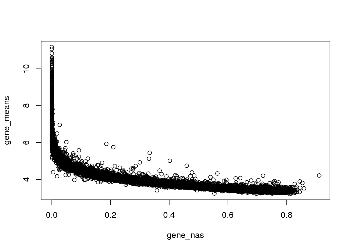

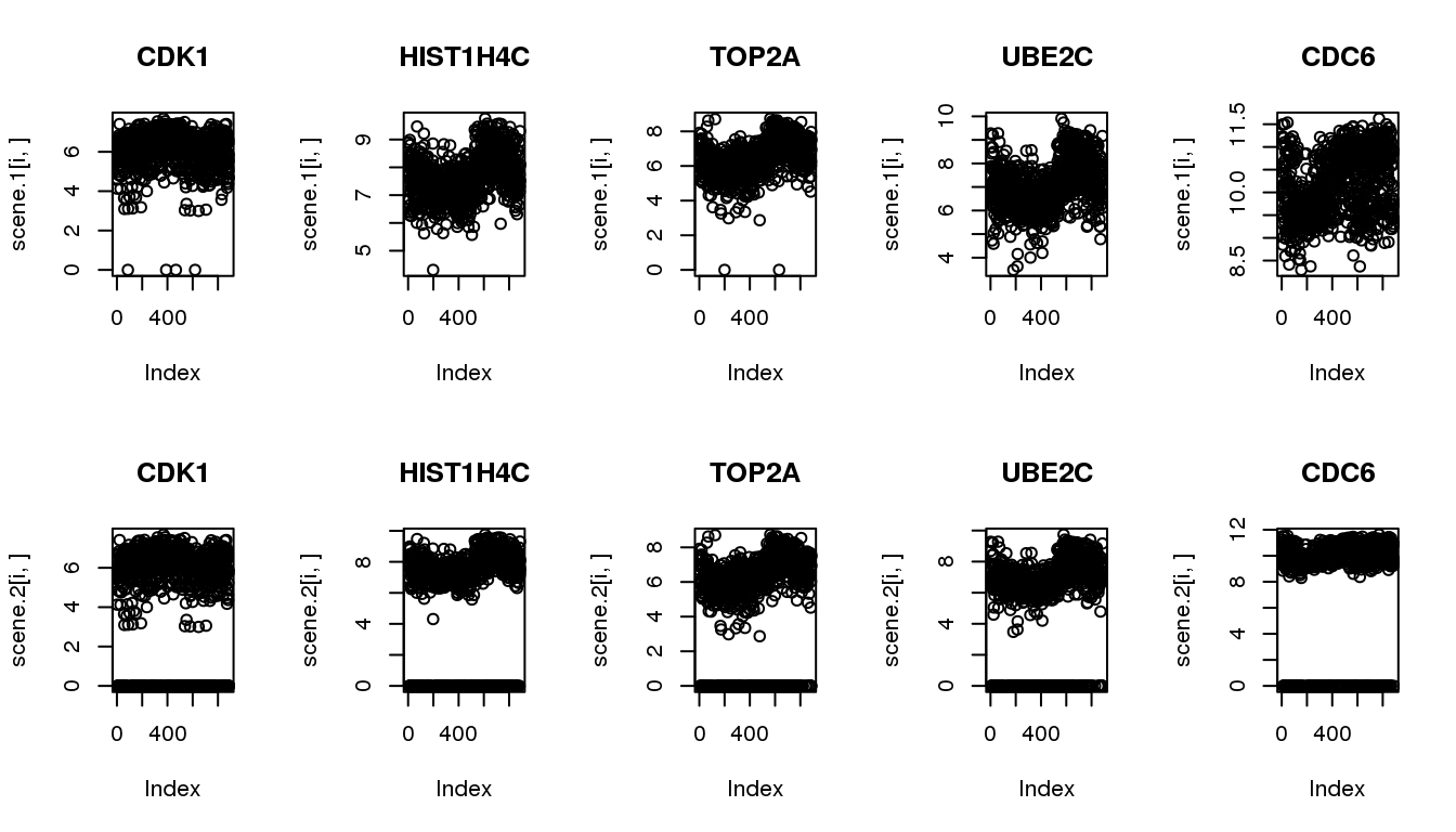
Make simulated data from the 5 identified cyclical genes

The goal of simulation is to compare the methods in their ability to recover cyclical patterns despite of zero observations.

1. Scenario 1: original data

2. Scenario 2: subsample to include 20% missing

N <- ncol(log2cpm.all)
scene.1 <- cycles.log2cpm
scene.2 <- do.call(rbind, lapply(1:nrow(cycles.log2cpm), function(g) {
  yy <- cycles.log2cpm[g,]
  numzeros <- round(N*0.2)
  numzeros <- numzeros - sum(yy==0)
  which.nonzero <- which(yy!=0)
  ii.zeros <- sample(which.nonzero,numzeros, replace = F)
  yy[ii.zeros] <- 0
  return(yy)
}))


par(mfrow=c(2,5))
for (i in 1:5) {
  plot(scene.1[i,], main = cycles$hgnc_symbol[i])
}
for (i in 1:5) {
  plot(scene.2[i,], main = cycles$hgnc_symbol[i])
}

out.1 <- lapply(1:5, function(i) {
  yy <- scene.2[i,]
  theta.sam <- theta
  out.trend <- fit.trendfilter(yy=yy, pos.yy=c(1:length(yy)))

  return(list(yy.sam=yy,
              theta.sam=theta.sam,
              out.trend=out.trend))
})

out.2 <- lapply(1:5, function(i) {
  yy <- scene.2[i,]
  out.trend <- fit.trendfilter.includezero(yy=yy, pos.yy=c(1:length(yy)))

  return(list(yy.sam=yy,
              theta.sam=theta,
              out.trend=out.trend))
})

saveRDS(out.1, file = "../output/npreg-trendfilter-prelim.Rmd/out1.rds")
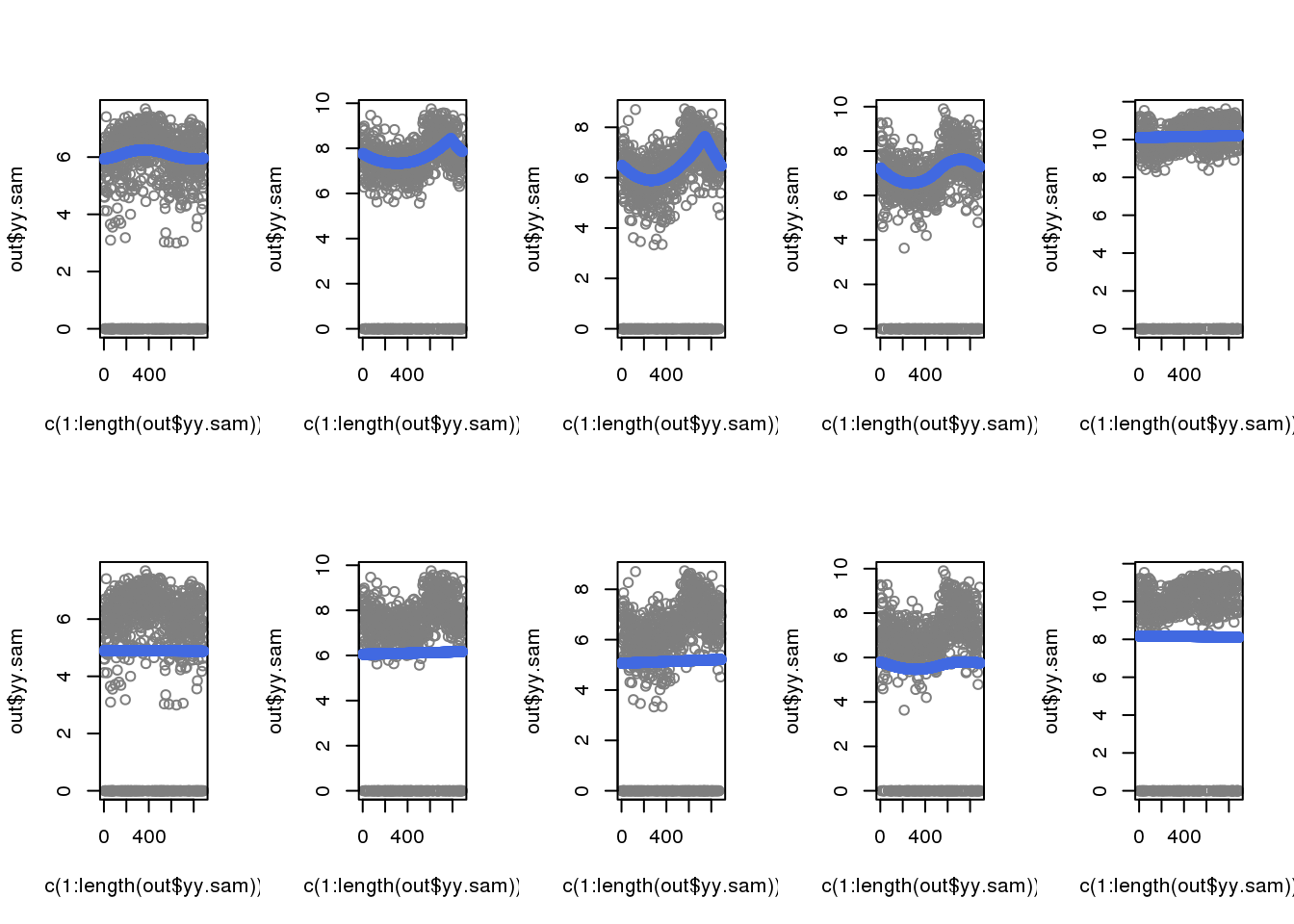
saveRDS(out.2, file = "../output/npreg-trendfilter-prelim.Rmd/out2.rds")

out.1 <- readRDS(file = "../output/npreg-trendfilter-prelim.Rmd/out1.rds")
out.2 <- readRDS(file = "../output/npreg-trendfilter-prelim.Rmd/out2.rds")

par(mfrow=c(2,5))
for (i in 1:5) {
  out <- out.1[[i]]
  plot(c(1:length(out$yy.sam)), out$yy.sam, col = "gray50")
  with(out$out.trend, 
       points(trend.pos, trend.yy, col = "royalblue"), cex=.5, pch=16)
}
for (i in 1:5) {
  out <- out.2[[i]]
  plot(c(1:length(out$yy.sam)), out$yy.sam, col = "gray50")
  with(out$out.trend, 
       points(trend.pos, trend.yy, col = "royalblue"), cex=.5, pch=16)
}

Session information

sessionInfo()

R version 3.4.1 (2017-06-30)
Platform: x86_64-redhat-linux-gnu (64-bit)
Running under: Scientific Linux 7.2 (Nitrogen)

Matrix products: default
BLAS/LAPACK: /usr/lib64/R/lib/libRblas.so

locale:
 [1] LC_CTYPE=en_US.UTF-8       LC_NUMERIC=C              
 [3] LC_TIME=en_US.UTF-8        LC_COLLATE=en_US.UTF-8    
 [5] LC_MONETARY=en_US.UTF-8    LC_MESSAGES=en_US.UTF-8   
 [7] LC_PAPER=en_US.UTF-8       LC_NAME=C                 
 [9] LC_ADDRESS=C               LC_TELEPHONE=C            
[11] LC_MEASUREMENT=en_US.UTF-8 LC_IDENTIFICATION=C       

attached base packages:
[1] parallel  stats     graphics  grDevices utils     datasets  methods  
[8] base     

other attached packages:
 [1] biomaRt_2.34.2      genlasso_1.3        igraph_1.2.1       
 [4] Matrix_1.2-10       MASS_7.3-47         matrixStats_0.53.1 
 [7] dplyr_0.7.4         Biobase_2.38.0      BiocGenerics_0.24.0
[10] conicfit_1.0.4      geigen_2.1          pracma_2.1.4       
[13] circular_0.4-93    

loaded via a namespace (and not attached):
 [1] progress_1.1.2       lattice_0.20-35      htmltools_0.3.6     
 [4] stats4_3.4.1         yaml_2.1.18          blob_1.1.0          
 [7] XML_3.98-1.10        rlang_0.2.0          pillar_1.2.1        
[10] glue_1.2.0           DBI_0.8              bit64_0.9-7         
[13] bindrcpp_0.2         bindr_0.1.1          stringr_1.3.0       
[16] mvtnorm_1.0-7        evaluate_0.10.1      memoise_1.1.0       
[19] knitr_1.20           IRanges_2.12.0       curl_3.1            
[22] AnnotationDbi_1.40.0 Rcpp_0.12.16         backports_1.1.2     
[25] S4Vectors_0.16.0     bit_1.1-12           digest_0.6.15       
[28] stringi_1.1.7        grid_3.4.1           rprojroot_1.3-2     
[31] tools_3.4.1          bitops_1.0-6         magrittr_1.5        
[34] RCurl_1.95-4.10      tibble_1.4.2         RSQLite_2.0         
[37] pkgconfig_2.0.1      prettyunits_1.0.2    assertthat_0.2.0    
[40] rmarkdown_1.9        httr_1.3.1           R6_2.2.2            
[43] boot_1.3-19          git2r_0.21.0         compiler_3.4.1