Compare Coefficient of variation between individuals
Joyce Hsiao
2015-10-16
Last updated: 2015-12-11
Code version: 884b335605607bd2cf5c9a1ada1e345466388866
Objective
Previously, we used the entire set of data including all individuals and all batches to perform normalization of coefficient of variations (link1) and performed
In this document, we wil perform per gene differential analysis of coefficients of variations using only coefficients of variation from ENSG genes and also from QC-approved batches (no NA19098.r2).
Set up
library("data.table")
library("dplyr")
library("limma")
library("edgeR")
library("ggplot2")
library("grid")
library("zoo")
theme_set(theme_bw(base_size = 12))
source("functions.R")
Prepare data
Input annotation of only QC-filtered single cells
anno_qc <- read.table("../data/annotation-filter.txt", header = TRUE,
                   stringsAsFactors = FALSE)
head(anno_qc)
individual replicate well batch sample_id
1 NA19098 r1 A01 NA19098.r1 NA19098.r1.A01
2 NA19098 r1 A02 NA19098.r1 NA19098.r1.A02
3 NA19098 r1 A04 NA19098.r1 NA19098.r1.A04
4 NA19098 r1 A05 NA19098.r1 NA19098.r1.A05
5 NA19098 r1 A06 NA19098.r1 NA19098.r1.A06
6 NA19098 r1 A07 NA19098.r1 NA19098.r1.A07Remove NA19098.r2
is_include <- anno_qc$batch != "NA19098.r2"
anno_qc_filter <- anno_qc[which(is_include), ]
Import endogeneous gene molecule counts that are QC-filtered, CPM-normalized, ERCC-normalized, and also processed to remove unwanted variation from batch effet. ERCC genes are removed from this file.
molecules_ENSG <- read.table("../data/molecules-final.txt", header = TRUE, stringsAsFactors = FALSE)
molecules_ENSG <- molecules_ENSG[ , is_include]
Input moleclule counts before log2 CPM transformation. This file is used to compute percent zero-count cells per sample.
molecules_sparse <- read.table("../data/molecules-filter.txt", header = TRUE, stringsAsFactors = FALSE)

molecules_sparse <- molecules_sparse[grep("ENSG", rownames(molecules_sparse)), ]
stopifnot( all.equal(rownames(molecules_ENSG), rownames(molecules_sparse)) )
Normalize coefficient of variation
Compute coefficient of variation.
# Compute CV and mean of normalized molecule counts (take 2^(log2-normalized count))

molecules_cv_batch_ENSG <-
  lapply(1:length(unique(anno_qc_filter$batch)), function(per_batch) {
      molecules_per_batch <- 2^molecules_ENSG[ , unique(anno_qc_filter$batch) == unique(anno_qc_filter$batch)[per_batch] ]
      mean_per_gene <- apply(molecules_per_batch, 1, mean, na.rm = TRUE)
      sd_per_gene <- apply(molecules_per_batch, 1, sd, na.rm = TRUE)
      cv_per_gene <- data.frame(mean = mean_per_gene,
                                sd = sd_per_gene,
                                cv = sd_per_gene/mean_per_gene)
      rownames(cv_per_gene) <- rownames(molecules_ENSG)

      # cv_per_gene <- cv_per_gene[rowSums(is.na(cv_per_gene)) == 0, ]
      cv_per_gene$batch <- unique(anno_qc_filter$batch)[per_batch]

      # Add sparsity percent
      molecules_sparse_per_batch <- molecules_sparse[ , unique(anno_qc_filter$batch) == unique(anno_qc_filter$batch)[per_batch]]
      cv_per_gene$sparse <- rowMeans(as.matrix(molecules_sparse_per_batch) == 0)

      return(cv_per_gene)
      })
names(molecules_cv_batch_ENSG) <- unique(anno_qc_filter$batch)

sapply(molecules_cv_batch_ENSG, dim)
NA19098.r1 NA19098.r3 NA19101.r1 NA19101.r2 NA19101.r3 NA19239.r1
[1,] 10564 10564 10564 10564 10564 10564
[2,] 5 5 5 5 5 5
NA19239.r2 NA19239.r3
[1,] 10564 10564
[2,] 5 5Merge summary data.frames.
df_ENSG <- do.call(rbind, molecules_cv_batch_ENSG)Compute rolling medians across all samples.
# Compute a data-wide coefficient of variation on CPM normalized counts.
data_cv_ENSG <- apply(2^molecules_ENSG, 1, sd)/apply(2^molecules_ENSG, 1, mean)

# Order of genes by mean expression levels
order_gene <- order(apply(2^molecules_ENSG, 1, mean))

# Rolling medians of log10 squared CV by mean expression levels
roll_medians <- rollapply(log10(data_cv_ENSG^2)[order_gene], width = 50, by = 25,
                         FUN = median, fill = list("extend", "extend", "NA") )
ii_na <- which( is.na(roll_medians) )
roll_medians[ii_na] <- median( log10(data_cv_ENSG^2)[order_gene][ii_na] )

names(roll_medians) <- rownames(molecules_ENSG)[order_gene]


# re-order rolling medians
reorder_gene <- match(rownames(molecules_ENSG), names(roll_medians) )
roll_medians <- roll_medians[ reorder_gene ]

stopifnot( all.equal(names(roll_medians), rownames(molecules_ENSG) ) )
Compute adjusted coefficient of variation.
# adjusted coefficient of variation on log10 scale
log10cv2_adj_ENSG <-
  lapply(1:length(molecules_cv_batch_ENSG), function(per_batch) {
    foo <- log10(molecules_cv_batch_ENSG[[per_batch]]$cv^2) - roll_medians
    return(foo)
})
df_ENSG$log10cv2_adj_ENSG <- do.call(c, log10cv2_adj_ENSG)
limma
We use the lmFit function in the limma package to fit linear models comparing coefficients of variations between individuals for all genes. lmFit provides a fast algorithm for least-square estimation, when design matrix is the same for all genes.
library(limma)

df_limma <- matrix(df_ENSG$log10cv2_adj_ENSG,
                      nrow = nrow(molecules_ENSG), ncol = 8, byrow = FALSE)

design <- data.frame(individual = factor(rep(unique(anno_qc_filter$individual), each = 3) ),
                     rep = factor(rep(c(1:3), times = 3)) )
design <- design[ with(design, !(individual == "NA19098" & rep == "2")), ]

colnames(df_limma) <- with(design, paste0(individual, rep))

fit_limma <- lmFit(df_limma, design = model.matrix( ~ individual, data = design))
fit_limma <- eBayes(fit_limma)
Voom plot of all genes
voom(10^df_limma, design = model.matrix(~individual, data = design),
     plot = TRUE)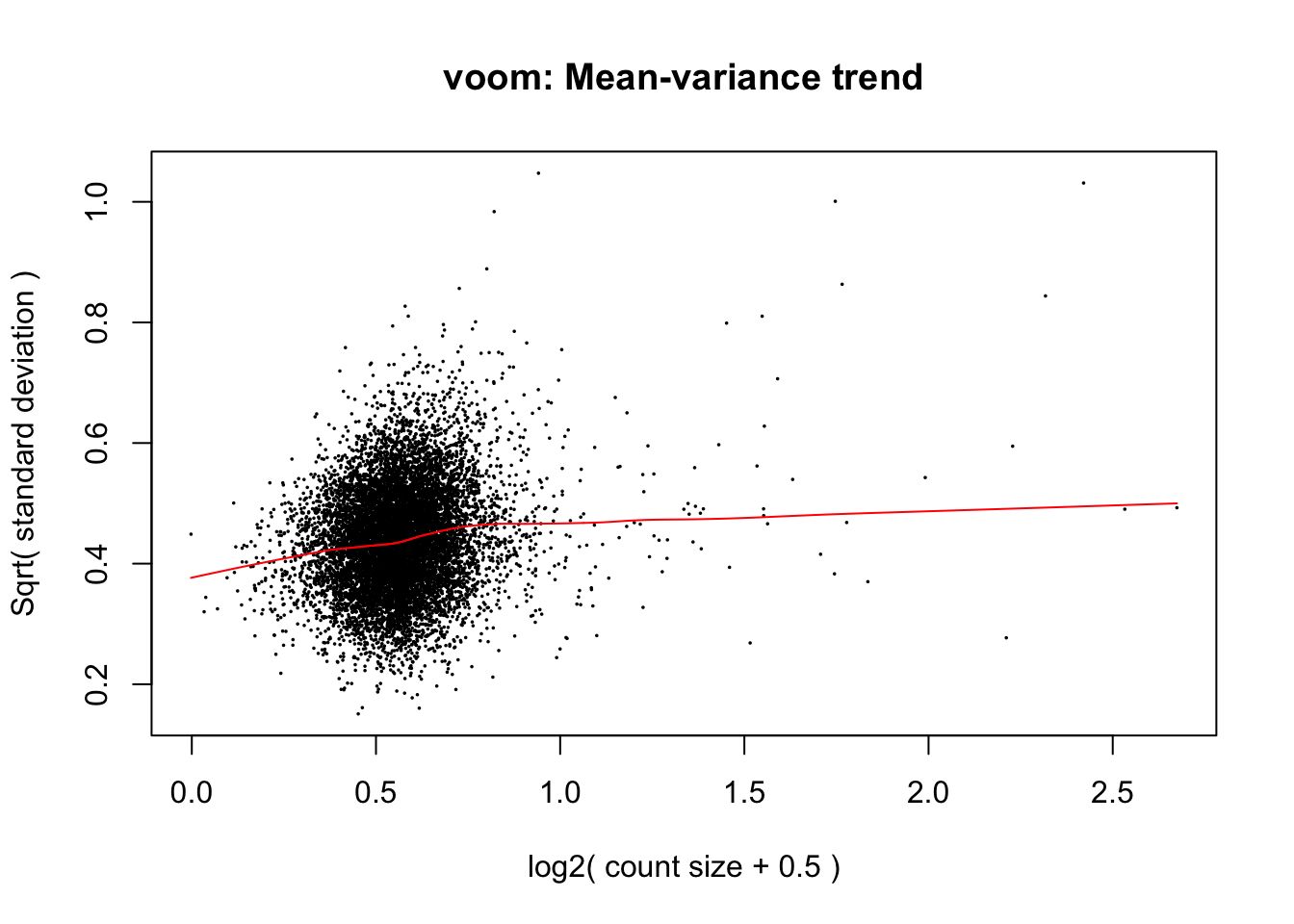
An object of class "EList"
$E
     NA190981 NA190983 NA191011 NA191012 NA191013 NA192391 NA192392
[1,] 6.667693 7.744440 7.177290 6.473759 6.768223 7.195293 7.179695
[2,] 6.789123 6.673820 6.865137 7.371818 7.297338 7.050406 7.293339
[3,] 7.087622 7.305000 7.291008 7.291007 7.060775 7.128955 7.054246
[4,] 6.814275 6.953216 6.791595 6.683958 6.650781 7.190253 6.694229
[5,] 6.548134 6.853805 6.959224 6.833469 6.959080 6.990432 6.985725
     NA192393
[1,] 7.155782
[2,] 6.936526
[3,] 7.397030
[4,] 6.654184
[5,] 6.864486
10559 more rows ...

$weights
         [,1]     [,2]     [,3]     [,4]     [,5]     [,6]     [,7]
[1,] 21.19654 27.72352 36.54855 36.64173 36.81388 26.20812 28.69949
[2,] 30.72420 43.71464 25.91773 26.01468 26.19418 28.87147 30.03071
[3,] 21.17937 28.01805 24.58450 24.65286 24.77921 25.47428 28.39366
[4,] 28.01208 36.17196 41.18261 41.29711 41.50874 35.11042 38.24292
[5,] 31.38078 45.54575 32.25810 32.33482 32.47651 31.48786 34.02597
         [,8]
[1,] 26.23264
[2,] 28.88002
[3,] 25.49795
[4,] 35.13233
[5,] 31.50386
10559 more rows ...

$design
  (Intercept) individualNA19101 individualNA19239
1           1                 0                 0
3           1                 0                 0
4           1                 1                 0
5           1                 1                 0
6           1                 1                 0
7           1                 0                 1
8           1                 0                 1
9           1                 0                 1
attr(,"assign")
[1] 0 1 1
attr(,"contrasts")
attr(,"contrasts")$individual
[1] "contr.treatment"


$targets
          lib.size
NA190981 12460.437
NA190983 10031.687
NA191011 10519.534
NA191012 10503.758
NA191013 10474.806
NA192391 10481.101
NA192392  9966.833
NA192393 10477.171
limma unmoderated F-test p-value
hist(fit_limma$F.p.value, breaks = 100, main = "F-test p-value")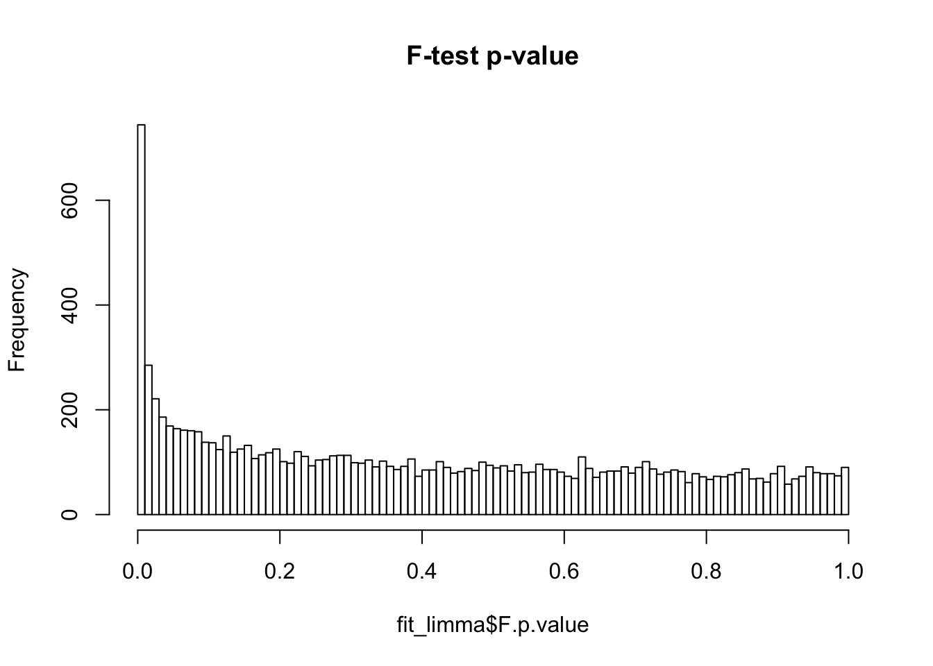
False discover control adjutment.
F.p.adj <- p.adjust(fit_limma$F.p.value, method = "fdr")
summary(F.p.adj)
Min. 1st Qu. Median Mean 3rd Qu. Max.
0.0000 0.4781 0.7170 0.6528 0.8836 0.9996 hist(F.p.adj, main = "False discovery rate", xlab = "FDR")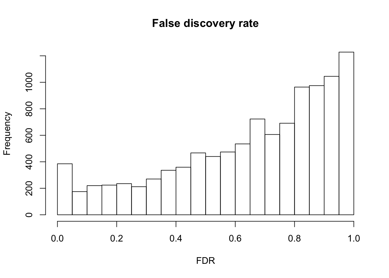
Cutoffs
df_cuts <- data.frame(cuts = c(.001, .01, .05, .1, .15, .2))
df_cuts$sig_count <- sapply(1:6, function(per_cut) {
                    sum(F.p.adj < df_cuts$cuts[per_cut] )
                    })
df_cuts
cuts sig_count
1 0.001 91
2 0.010 192
3 0.050 385
4 0.100 560
5 0.150 780
6 0.200 1004P-value before versus after false discovery adjustment.
plot(y = F.p.adj, x = fit_limma$F.p.value,
     xlab = "F-test p-value", ylab = "FDR")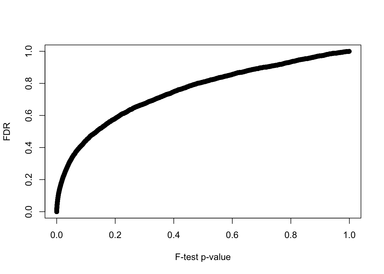
P-value and sparsity
df_sparse <- rowMeans(matrix(df_ENSG$sparse, nrow = nrow(molecules_ENSG), ncol = 8,
                      byrow = FALSE) )

plot(x = df_sparse, y = log10(fit_limma$F.p.value),
     xlab = "Average percent of zero-count cells",
     ylab = "log10(p-value of F-test)",
     main = "CV and sparsity of all genes", col = "grey60")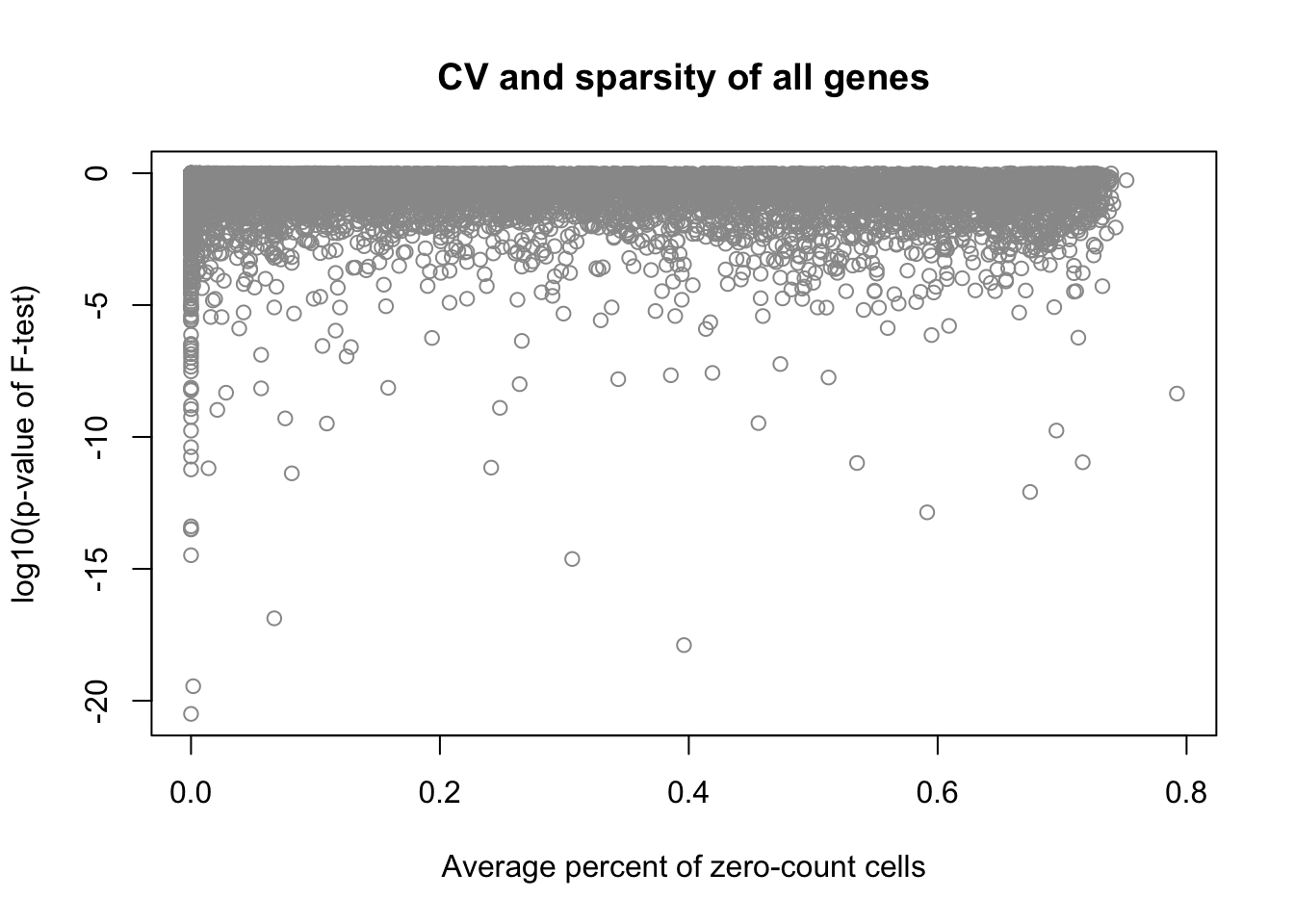
Correlation between mean sparsity rate and p-value.
cor(df_sparse, fit_limma$F.p.value, method = "spearman")[1] -0.1791479CPM density distributions of significant genes
Rank genes by FDR.
order_limma <- order(F.p.adj)

ggplot(data.frame(values = unlist(molecules_ENSG[order_limma[1],] ),
                  individual = factor(anno_qc_filter$individual),
                  replicate = factor(anno_qc_filter$replicate),
                  batch = factor(anno_qc_filter$batch), check.rows = F)
       , aes(x = values)) +
  geom_density(aes(group = batch, col = individual)) +
  ggtitle(paste("The most significant gene", rownames(molecules_ENSG)[order_limma[1]]) )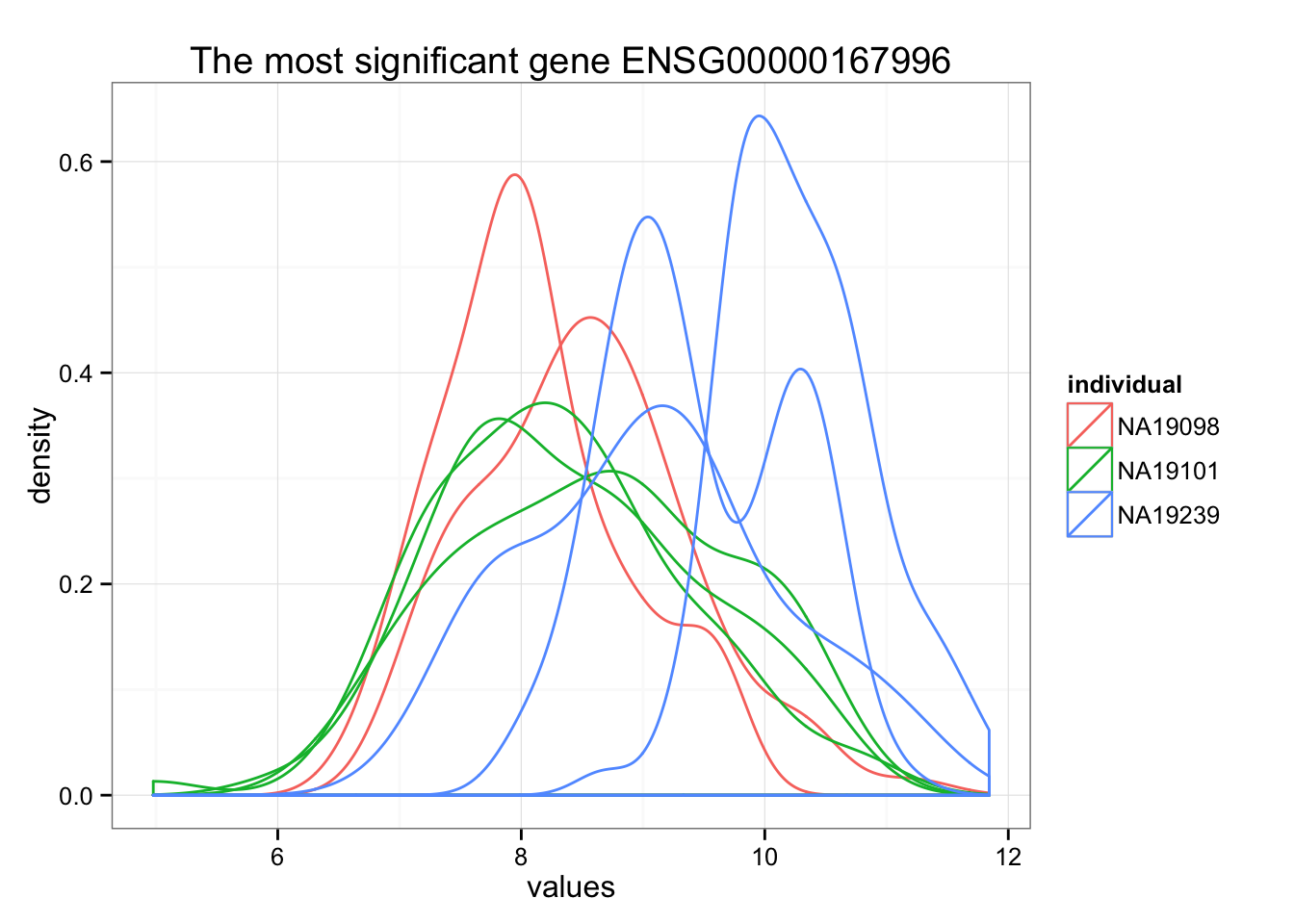
ggplot(data.frame(values = unlist(molecules_ENSG[order_limma[2],] ),
                  individual = factor(anno_qc_filter$individual),
                  replicate = factor(anno_qc_filter$replicate),
                  batch = factor(anno_qc_filter$batch), check.rows = F), aes(x = values)) +
  geom_density(aes(group = batch, col = individual)) +
  ggtitle(paste("The second significant gene", rownames(molecules_ENSG)[order_limma[2]]) )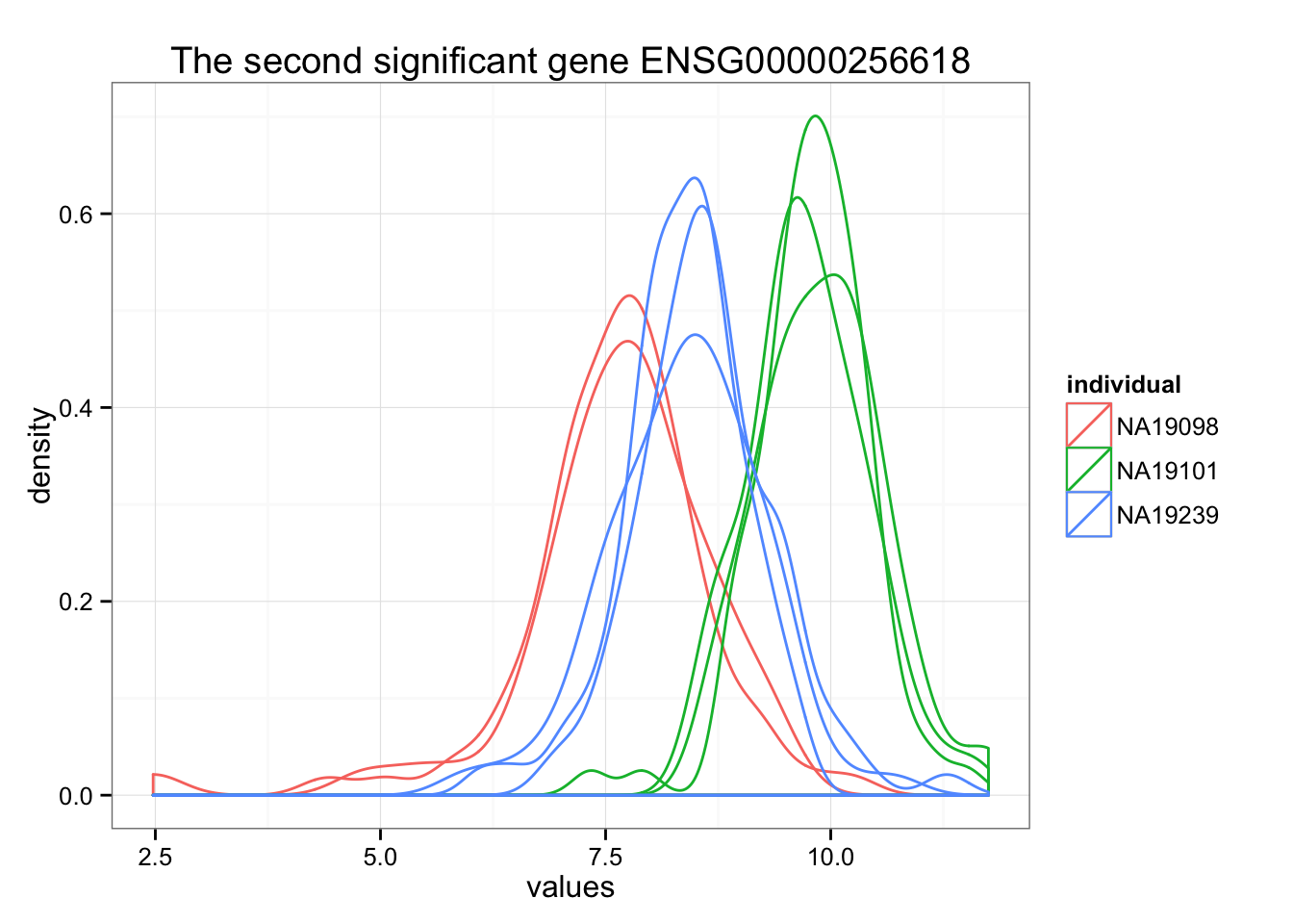
ggplot(data.frame(values = unlist(molecules_ENSG[order_limma[3],] ),
                  individual = factor(anno_qc_filter$individual),
                  replicate = factor(anno_qc_filter$replicate),
                  batch = factor(anno_qc_filter$batch), check.rows = F), aes(x = values)) +
  geom_density(aes(group = batch, col = individual)) +
  ggtitle(paste("The third significant gene", rownames(molecules_ENSG)[order_limma[3]]) )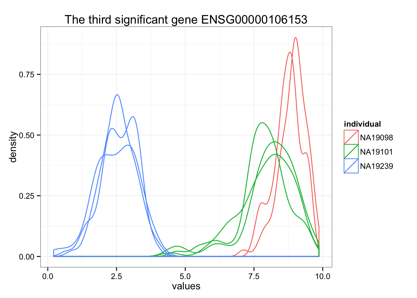
Session information
sessionInfo()R version 3.2.1 (2015-06-18)
Platform: x86_64-apple-darwin13.4.0 (64-bit)
Running under: OS X 10.10.5 (Yosemite)
locale:
[1] en_US.UTF-8/en_US.UTF-8/en_US.UTF-8/C/en_US.UTF-8/en_US.UTF-8
attached base packages:
[1] grid stats graphics grDevices utils datasets methods
[8] base
other attached packages:
[1] zoo_1.7-12 ggplot2_1.0.1 edgeR_3.10.5 limma_3.24.15
[5] dplyr_0.4.3 data.table_1.9.6 knitr_1.11
loaded via a namespace (and not attached):
[1] Rcpp_0.12.2 magrittr_1.5 MASS_7.3-45 munsell_0.4.2
[5] lattice_0.20-33 colorspace_1.2-6 R6_2.1.1 stringr_1.0.0
[9] plyr_1.8.3 tools_3.2.1 parallel_3.2.1 gtable_0.1.2
[13] DBI_0.3.1 htmltools_0.2.6 yaml_2.1.13 assertthat_0.1
[17] digest_0.6.8 reshape2_1.4.1 formatR_1.2.1 evaluate_0.8
[21] rmarkdown_0.8.1 labeling_0.3 stringi_1.0-1 scales_0.3.0
[25] chron_2.3-47 proto_0.3-10