Diminishing returns of sequencing depth

Introduction

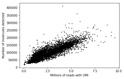
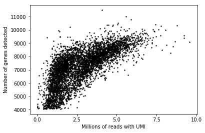
We previously observed that the number of genes/molecules detected does not saturate with increasing sequencing depth.

Here, we quantify the potential gain in additional sequencing of the samples in terms of number of molecules and number of genes detected.

Analysis

annotations.shape

(5012, 40)

plt.clf()
plt.scatter(annotations['umi'], annotations['mol_hs'], color='k', s=2)
plt.xticks(np.linspace(0, 1, 5) * 1e7, np.linspace(0, 1, 5) * 10)
plt.xlabel('Millions of reads with UMI')
_ = plt.ylabel('Number of molecules detected')

plt.clf()
plt.scatter(annotations['umi'], annotations['detect_hs'], color='k', s=2)
plt.xticks(np.linspace(0, 1, 5) * 1e7, np.linspace(0, 1, 5) * 10)
plt.xlabel('Millions of reads with UMI')
_ = plt.ylabel('Number of genes detected')

To see whether the trend is different per individual, fit a linear regression per individual:

def _lm(x):
  m = lm.LinearRegression(fit_intercept=True).fit(x['umi'].values.reshape(-1, 1), x['mol_hs'].values)
  rss = np.square(x['mol_hs'].values - m.predict(x['umi'].values.reshape(-1, 1))).sum()
  sigma2 = rss / x.shape[0]
  var = x['umi'].var()
  se = sigma2 / var
  return pd.Series({'beta': m.coef_[0], 'se': se, 'intercept': m.intercept_})

beta = annotations.groupby('chip_id').apply(_lm).sort_index()

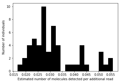
Plot the distribution of regression coefficients:

plt.clf()
plt.hist(beta['beta'].values, color='k', bins=20)
plt.xlabel('Estimated number of molecules detected per additional read')
_ = plt.ylabel('Number of individuals')

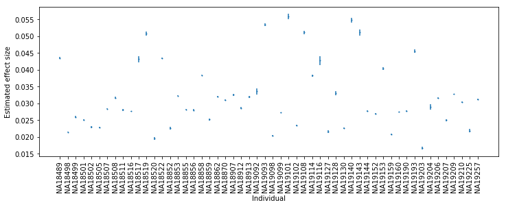
plt.clf()
plt.gcf().set_size_inches(12, 4)
plt.errorbar(x=np.arange(beta.shape[0]), y=beta['beta'].values, yerr=beta['se'].values, ls='', marker='o', ms=1)
plt.xticks(np.arange(beta.shape[0]), beta.index, rotation=90)
plt.xlabel('Individual')
_ = plt.ylabel('Estimated effect size')