Power to detect QTLs in single cell data

Introduction

We previously found that our study lost power to detect eQTLs, and was underpowered to directly detect dQTLs.

Here, we perform the following analyses:

We derive the power function accounting for measurement error
We show that dQTL effects are larger than eQTL effects (in terms of log fold change)
We show that PVE explains lack of power to detect dQTLs (rather than measurement error)
We solve for the sample size required to achieve 80% power to detect the strongest dQTLs

Empirical power calculation

Differential dispersion

Perform a nested model comparison for each gene \(k\), comparing the model:

\[ r_{ijk} \sim \mathrm{ZINB}(\pi_{ik}, \mu_{ik}, \phi_{ik}) \]

against the model:

\[ r_{ijk} \sim \mathrm{ZINB}(\pi_{ik}, \mu_{ik}, \phi_{i}) \]

def lrt(umi, onehot, design, size_factor):
  _, _, _, llik0 = fit(
    umi=umi.values.T.astype(np.float32),
    onehot=onehot.astype(np.float32),
    design=design.astype(np.float32),
    size_factor=size_factor.astype(np.float32),
    fit_null=True,
    return_llik=True,
    learning_rate=5e-2,
    max_epochs=4000)
  _, _, _, llik1 = fit(
    umi=umi.values.T.astype(np.float32),
    onehot=onehot.astype(np.float32),
    design=design.astype(np.float32),
    size_factor=size_factor.astype(np.float32),
    return_llik=True,
    learning_rate=5e-2,
    max_epochs=4000)
  T = 2 * (llik1 - llik0)
  return T, st.chi2(1).logsf(T)

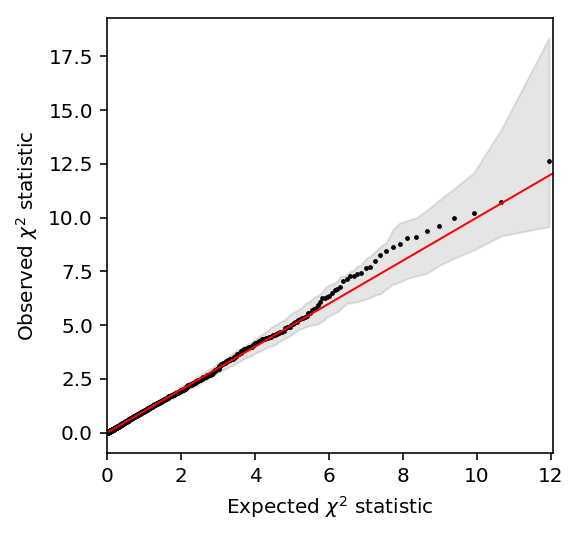
Null calibration via parametric bootstrap

Sample null data from the model, using empirical estimates of the parameters in the observed data.

<<zinb-imports>>
<<tf-imports>>
<<tf-zinb-impl>>
<<lrt-impl>>
<<sim-impl>>

log_mu = pd.read_table('/project2/mstephens/aksarkar/projects/singlecell-qtl/data/density-estimation/design1/zi2-log-mu.txt.gz', index_col=0, sep=' ')
log_phi = pd.read_table('/project2/mstephens/aksarkar/projects/singlecell-qtl/data/density-estimation/design1/zi2-log-phi.txt.gz', index_col=0, sep=' ')
logodds = pd.read_table('/project2/mstephens/aksarkar/projects/singlecell-qtl/data/density-estimation/design1/zi2-log-mu.txt.gz', index_col=0, sep=' ')
params = pd.DataFrame({'log_mu': log_mu['NA18507'],
                       'log_phi': log_phi['NA18507'],
                       'logodds': logodds['NA18507']},
                      index=log_mu.index)
params = params[params['log_mu'] > -10]
n = 100
umi = pd.DataFrame([simulate(2 * n, size=1e5, log_mu=log_mu, log_phi=log_phi, logodds=logodds)[0][:,0]
                    for _, (log_mu, log_phi, logodds) in params.iterrows() if log_mu > -10], index=params.index)
onehot = np.zeros((2 * n, 2))
onehot[:n,0] = 1
onehot[n:,1] = 1
design = np.zeros((2 * n, 1))
size_factor = 1e5 * np.ones((2 * n, 1))
T, P = lrt(umi, onehot, design, size_factor)
pd.DataFrame({'chi2': T, 'logp': P}, index=umi.index).to_csv('null-calibration-p.txt.gz', sep='\t', compression='gzip')

sbatch --partition=gpu --gres=gpu:1 --mem=16G --job-name=tf-lrt-null --output=tf-lrt-null-parametric.out
#!/bin/bash
source activate scqtl
python /project2/mstephens/aksarkar/projects/singlecell-qtl/code/tf-lrt-null-parametric.py

Submitted batch job 46322399

Read the results.

null_lrt = pd.read_table('/scratch/midway2/aksarkar/singlecell/power/null-calibration-p.txt.gz')
N = null_lrt.shape[0]

Report how many genes were simulated.

Estimate bootstrap CIs for the quantiles.

B = np.sort(st.chi2(1).rvs((N, 100)), axis=0)
ci = np.percentile(B, [2.5, 97.5], axis=1)

Plot the QQ-plot.

plt.clf()
plt.gcf().set_size_inches(4, 4)
grid = st.chi2(1).ppf(np.linspace(0, 1 - 1 / N, N))
plt.scatter(grid, null_lrt['chi2'].sort_values(), c='k', s=2)
plt.fill_between(grid, ci[0], ci[1], color='k', alpha=0.1)
lim = [0, 1.01 * grid.max()]
plt.plot(lim, lim, c='r', lw=1)
plt.xlim(lim)
plt.xlabel('Expected $\chi^2$ statistic')
_ = plt.ylabel('Observed $\chi^2$ statistic')

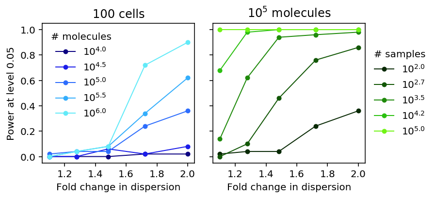
Power

Sample from the assumed model.

<<zinb-imports>>
<<tf-imports>>
<<tf-zinb-impl>>
<<lrt-impl>>
<<sim-impl>>

log_mu = pd.read_table('/project2/mstephens/aksarkar/projects/singlecell-qtl/data/density-estimation/design1/zi2-log-mu.txt.gz', index_col=0, sep=' ')
log_phi = pd.read_table('/project2/mstephens/aksarkar/projects/singlecell-qtl/data/density-estimation/design1/zi2-log-phi.txt.gz', index_col=0, sep=' ')
logodds = pd.read_table('/project2/mstephens/aksarkar/projects/singlecell-qtl/data/density-estimation/design1/zi2-log-mu.txt.gz', index_col=0, sep=' ')
params = pd.DataFrame({'log_mu': log_mu['NA18507'],
                       'log_phi': log_phi['NA18507'],
                       'logodds': logodds['NA18507']},
                      index=log_mu.index)
params = params[params['log_mu'] > -10].sample(n=50)

sample_sizes = np.geomspace(1e2, 1e5, 5).astype(int)
log_fold_changes = np.log(np.geomspace(1.1, 2, 5))
depths = np.geomspace(1e4, 1e6, 5)

result = []
for num_mols in depths:
  for log_fc in log_fold_changes:
    for num_samples in sample_sizes:
      umi = []
      for _, (log_mu, log_phi, logodds) in params.iterrows():
        umi.append(np.hstack([
          simulate(num_samples, size=num_mols, log_mu=log_mu, log_phi=log_phi, logodds=logodds)[0][:,0],
          simulate(num_samples, size=num_mols, log_mu=log_mu, log_phi=log_phi + log_fc, logodds=logodds)[0][:,0]
        ]))
      umi = pd.DataFrame(umi, index=params.index)
      onehot = np.zeros((umi.shape[1], 2))
      onehot[:num_samples,0] = 1
      onehot[num_samples:,1] = 1
      design = np.zeros((umi.shape[1], 1))
      size_factor = num_mols * np.ones((umi.shape[1], 1))
      T, P = lrt(umi, onehot, design, size_factor)
      result.append(pd.DataFrame({
        'num_mols': num_mols,
        'num_samples': num_samples,
        'log_fold_change': log_fc,
        'chi2': T,
        'logp': P}))
pd.concat(result).to_csv('lrt-power.txt.gz', sep='\t', compression='gzip')

sbatch --partition=gpu --gres=gpu:1 --mem=16G --job-name=tf-lrt-power --output=tf-lrt-power.out
#!/bin/bash
source activate scqtl
python /project2/mstephens/aksarkar/projects/singlecell-qtl/code/tf-lrt-power.py

Submitted batch job 46367157

sacct -j 46367157 -o Elapsed

   Elapsed 
---------- 
  06:59:58 
  06:59:58 
  06:59:58

Move the results to permanent storage.

rsync -FFau /scratch/midway2/aksarkar/singlecell/power/ /project2/mstephens/aksarkar/projects/singlecell-qtl/data/power/

Read the results.

lrt_results = (pd.read_table('/project2/mstephens/aksarkar/projects/singlecell-qtl/data/power/lrt-power.txt.gz', index_col=0)
             .reindex())
features = ['num_mols', 'num_samples', 'log_fold_change']
lrt_power = (lrt_results
             .groupby(features)
             .apply(lambda x: (np.exp(x['logp']) < 0.05).sum() / x.shape[0])
             .to_frame()
             .reset_index())

Plot the results.

plt.clf()
fig, ax = plt.subplots(1, 2, sharey=True)
fig.set_size_inches(5.5, 3)

num_samples = 100
groups = sorted(set(lrt_power['num_mols']))
for i, n in enumerate(groups):
  color = colorcet.cm['kbc']((i + .5) / len(groups))
  subset = lrt_power[np.logical_and(lrt_power['num_mols'] == n, lrt_power['num_samples'] == num_samples)]
  ax[0].plot(np.exp(subset['log_fold_change']), subset[0], lw=1, marker='.', ms=8, c=color, label='$10^{{{:.1f}}}$'.format(np.log(n) / np.log(10)))
ax[0].legend(title='# molecules', frameon=False)
ax[0].set_xlabel('Fold change in dispersion')
ax[0].set_ylabel('Power at level 0.05')
ax[0].set_title('100 cells')

num_mols = 1e5
grid = np.log(np.linspace(1.1, 2, 100))
groups = sorted(set(lrt_power['num_samples']))
for i, n in enumerate(groups):
  color = colorcet.cm['kgy']((i + .5) / len(groups))
  subset = lrt_power[np.logical_and(lrt_power['num_mols'] == num_mols, lrt_power['num_samples'] == n)]
  ax[1].plot(np.exp(subset['log_fold_change']), subset[0], lw=1, marker='.', ms=8, c=color, label='$10^{{{:.1f}}}$'.format(np.log(n) / np.log(10)))
ax[1].legend(title='# samples', frameon=False, loc='center left', bbox_to_anchor=(1, .5))
ax[1].set_xlabel('Fold change in dispersion')
ax[1].set_title('$10^5$ molecules')

fig.tight_layout()

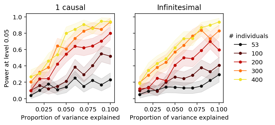
QTL discovery

We assume the phenotype is generated from \(m\) causal effects (out of \(p\) variants) following a linear model:

\[ \theta_i = \sum_j X_{ij} \beta_j + \epsilon_i \]

\[ \mathbb{E}[x_i] = 0, \mathbb{V}[x_i] = 1 \]

\[ \beta_j \sim N(0, 1) \text{ if \(j\) causal}\]

\[ \epsilon_i \sim N(0, \mathbb{V[X \beta]} (1 / h^2 - 1)) \]

def read_dosage(vcf, row, window=100000):
  records = list(vcf.query(row['#Chr'], row['start'] - window, row['start'] + window))
  if records:
    x = np.array([record[9:] for record in records]).astype(np.float).T
    x = pd.DataFrame(x, columns=[record[2] for record in records])
    return x
  else:
    return None

def read_vcf_geno(vcf, chrom, start, end):
  records = list(vcf.query(chrom, start, end))
  if records:
    x = (np.array([[_.split('/') for record in records for _ in record[9:]]])
         .reshape(len(records), -1, 2)
         .astype(float)
         .sum(axis=-1))
    return np.array(x).T
  else:
    return None

def generate_pheno(x, pve, m=None):
  x = x[:,np.logical_and(x.mean(axis=0) / 2 > 0.05, x.std(axis=0) > 0)]
  n, p = x.shape
  if p == 0:
    return None
  if m is None:
    theta = np.random.normal(size=p)
  else:
    theta = np.zeros(p)
    theta[np.random.choice(p, m, replace=False)] = np.random.normal(size=m)
  x -= x.mean(axis=0)
  x /= x.std(axis=0)
  y = x.dot(theta)
  y += np.random.normal(scale=np.sqrt(y.var() * (1 / pve - 1)), size=n)
  y -= y.mean()
  y /= y.std()
  return y.reshape(-1, 1)

def lm(x, y):
  n = y.shape[0]
  beta = x.T.dot(y) / n
  df = n - 1
  rss = ((y ** 2).sum() - beta ** 2 * n)
  sigma2 = rss / df
  se = np.sqrt(sigma2 / n)
  return beta, se

_sf = st.chi2(1).sf

def nominal_test(x, y):
  beta, se = lm(x, y)
  return _sf((beta / se) ** 2)

def beta_llik(theta, x):
  return -st.beta.logpdf(x, *theta).mean()

def permutation_test(x, y, num_trials=100):
  pval = nominal_test(x, y).min()
  null_pheno = y.copy()
  null_pvals = []
  for _ in range(num_trials):
    np.random.shuffle(null_pheno)
    null_pvals.append(nominal_test(x, null_pheno).min())
  null_pvals = np.array(null_pvals)
  theta = np.ones(2)
  opt = so.minimize(beta_llik, x0=theta, args=(null_pvals,))
  if opt.success:
    theta = opt.x
  else:
    # Method of moments
    theta = np.array([1, (1 / null_pvals.mean() - 1)])
    theta *= np.square(null_pvals.mean()) * ((1 - null_pvals.mean()) / null_pvals.var() - 1)
  return st.beta.cdf(pval, *theta)

def evaluate(vcf, eqtls, num_individuals, num_causal, pve, num_genes=100):
  query = eqtls.sample(n=num_genes)
  result = []
  for _, record in query.iterrows():
    # Important: GEUVADIS chromosomes are coded 1-22
    x = read_vcf_geno(vcf, record['chr'][3:], record['start'] - 100000, record['start'] + 100000)
    if x is None:
      continue
    y = None
    while y is None:
      # Important: rejection sampling is needed to get a subset of individuals
      # with enough variable SNPs
      keep = np.random.choice(x.shape[0], num_individuals, replace=False)
      z = x[keep]
      y = generate_pheno(z, pve=pve, m=num_causal)
    pval = permutation_test(z, y)
    result.append({
      'gene': record.name,
      'num_individuals': z.shape[0],
      'num_snps': z.shape[1],
      'num_causal': num_causal,
      'pve': pve,
      'pval': pval})
  return pd.DataFrame.from_dict(result)

QC the GEUVADIS genotypes.

sbatch --partition=broadwl --mem=4G --job-name=plink -a 1-22
#!/bin/bash
plink --memory 4000 --vcf /project/compbio/geuvadis/genotypes/GEUVADIS.chr${SLURM_ARRAY_TASK_ID}.*.vcf.gz --maf 0.05 --geno 0.01 --make-bed --out geuvadis-$SLURM_ARRAY_TASK_ID

Submitted batch job 46479117

Write out and index the QC'ed VCF.

sbatch --partition=broadwl --mem=4G --job-name=geuvadis --out=geuvadis.out
#!/bin/bash
set -e
module load parallel
source activate scqtl
parallel echo geuvadis-{} ::: $(seq 1 22) >merge.txt
plink --memory 4000 --merge-list merge.txt --recode vcf-iid --out geuvadis
bgzip geuvadis.vcf
tabix geuvadis.vcf.gz

Submitted batch job 46404341

Run the power calculation on 28 CPUs.

<<power-imports>>
<<eqtl-sim-impl>>

vcf = tabix.open('/scratch/midway2/aksarkar/singlecell/power/geuvadis.vcf.gz')
# Restrict to genes where we previously successfully mapped eQTLs
eqtls = pd.read_table('/project2/mstephens/aksarkar/projects/singlecell-qtl/data/scqtl-mapping/pooled.txt.gz', sep=' ', index_col=0).dropna()

args = [(vcf, eqtls, n, m, pve)
        for n in (53, 100, 200, 300, 400)
        for m in (1, None)
        for pve in np.linspace(0.01, 0.1, 10)]

np.random.seed(0)
result = [evaluate(*a) for a in args]
pd.concat(result).to_csv('eqtl-power.txt.gz', compression='gzip', sep='\t')

sbatch --partition=broadwl -n1 -c28 --exclusive --time=3:00:00 --mem=16G --job-name=eqtl-power --output=eqtl-power.out
#!/bin/bash
source activate scqtl
python /project2/mstephens/aksarkar/projects/singlecell-qtl/code/eqtl-power.py

Submitted batch job 46541021

Read the results.

# Important: we used None for infinitesimal, which gets parsed as missing
qtl_results = pd.read_table('/project2/mstephens/aksarkar/projects/singlecell-qtl/data/power/eqtl-power.txt.gz', index_col=0).fillna(-1)
qtl_results['sig'] = qtl_results.apply(lambda x: x['pval'] < 0.05, axis=1).astype(int)
qtl_power = (qtl_results
             .groupby(['num_individuals', 'num_causal', 'pve'])['sig']
             .agg([np.mean, np.std])
             .reset_index()
             .rename(columns={'mean': 'power', 'std': 'se'}))
qtl_power['se'] /= 10

Plot the results.

plt.clf()
fig, ax = plt.subplots(1, 2, sharey=True)
fig.set_size_inches(5.5, 3)
groups = sorted(set(qtl_power['num_individuals']))
for i, m in enumerate([1, -1]):
  for n in groups:
    subset = np.logical_and(qtl_power['num_individuals'] == n, qtl_power['num_causal'] == m)
    color = colorcet.cm['linear_kry_5_95_c72']((n - 53) / (max(groups) - 25))
    ax[i].plot(qtl_power.loc[subset, 'pve'],
               qtl_power.loc[subset, 'power'],
               marker='.', c=color, lw=1, ms=8, label=n)
    ax[i].fill_between(qtl_power.loc[subset, 'pve'],
                       qtl_power.loc[subset, 'power'] - 1.96 * qtl_power.loc[subset, 'se'],
                       qtl_power.loc[subset, 'power'] + 1.96 * qtl_power.loc[subset, 'se'],
                       color=color, alpha=0.1)
ax[0].set_title('1 causal')
ax[1].set_title('Infinitesimal')
ax[0].set_ylabel('Power at level 0.05')
ax[-1].legend(title='# individuals', frameon=False, loc='center left', bbox_to_anchor=(1, .5))

for a in ax:
  a.set_xlabel('Proportion of variance explained')
  a.set_xlim(0.005, .105)

fig.tight_layout()

Distribution of effect sizes.

Use ash to estimate the distribution of true effect sizes across all genes. We need to compute regression standard errors ourselves.

def run_nominal_pass(vcf, pheno, header, std=True, cov=None):
  # Annihilator matrix I - X X^+
  M = None
  result = []
  for _, record in pheno.iterrows():
    x = read_dosage(vcf, record)
    if x is not None:
      x.index = header
      y = record
      x, y = x.align(y, axis='index', join='inner')
      x -= x.mean(axis=0)
      x /= x.std(axis=0)
      if M is None and cov is not None:
        cov = cov.T.align(y, axis='index', join='inner')[0]
        C = np.array(cov - cov.mean(axis=0))
        M = np.eye(C.shape[0]) - C.dot(np.linalg.pinv(C))
      y = y.astype(float).values.reshape(-1, 1)
      if M is not None:
        y = M.dot(y)
      y -= y.mean()
      if std:
        y /= y.std()
      beta, se = lm(x, y)
      result.append(pd.DataFrame({'gene': record.name, 'beta': beta[0], 'se': se[0]}))
  return pd.concat(result)

<<power-imports>>
import argparse
<<eqtl-sim-impl>>
<<nominal-pass-def>>

parser = argparse.ArgumentParser()
parser.add_argument('--vcf', required=True)
parser.add_argument('--pheno', required=True)
parser.add_argument('--cov')
parser.add_argument('--no-std', action='store_true')
parser.add_argument('--out', default=None)
args = parser.parse_args()

vcf = tabix.open(args.vcf)
header = pd.read_table(args.vcf, skiprows=2, nrows=1, header=0).columns[9:]
pheno = pd.read_table(args.pheno, index_col=4)
if args.cov is not None:
  cov = pd.read_table(args.cov, sep=r'\s+', engine='python', index_col=0)
else:
  cov = None

result = run_nominal_pass(vcf, pheno, header, cov=cov, std=not args.no_std)
if args.out is None:
  out = 'nominal-pass.txt.gz'
else:
  out = args.out
result.to_csv(out, sep='\t', compression='gzip')

sbatch --partition=broadwl -a 1-7 -n1 -c28 --exclusive --job-name=nominal --out nominal.out --time=60:00
#!/bin/bash
source activate scqtl
tasks=(
    "python /project2/mstephens/aksarkar/projects/singlecell-qtl/code/qtl-nominal.py --vcf /scratch/midway2/aksarkar/singlecell/scqtl-mapping/yri-120-dosages.vcf.gz --pheno /scratch/midway2/aksarkar/singlecell/scqtl-mapping/log_phi.bed.gz --out log_phi.txt.gz"
    "python /project2/mstephens/aksarkar/projects/singlecell-qtl/code/qtl-nominal.py --vcf /scratch/midway2/aksarkar/singlecell/scqtl-mapping/yri-120-dosages.vcf.gz --pheno /project2/mstephens/aksarkar/projects/singlecell-qtl/data/scqtl-mapping/mean.bed.gz --cov /project2/mstephens/aksarkar/projects/singlecell-qtl/data/scqtl-mapping/mean-covars.txt --out mean.txt.gz"
    "python /project2/mstephens/aksarkar/projects/singlecell-qtl/code/qtl-nominal.py --vcf /scratch/midway2/aksarkar/singlecell/scqtl-mapping/yri-120-dosages.vcf.gz --pheno /project2/mstephens/aksarkar/projects/singlecell-qtl/data/scqtl-mapping/bulk.bed.gz --cov /project2/mstephens/aksarkar/projects/singlecell-qtl/data/scqtl-mapping/bulk-covars.txt --out bulk.txt.gz"
    "python /project2/mstephens/aksarkar/projects/singlecell-qtl/code/qtl-nominal.py --vcf /scratch/midway2/aksarkar/singlecell/scqtl-mapping/yri-120-dosages.vcf.gz --pheno /scratch/midway2/aksarkar/singlecell/scqtl-mapping/resid.bed.gz --cov /scratch/midway2/aksarkar/singlecell/scqtl-mapping/resid-covars.txt --out resid.txt.gz"
    "python /project2/mstephens/aksarkar/projects/singlecell-qtl/code/qtl-nominal.py --vcf /scratch/midway2/aksarkar/singlecell/scqtl-mapping/yri-120-dosages.vcf.gz --pheno /scratch/midway2/aksarkar/singlecell/scqtl-mapping/cv_resid.bed.gz --out cv_resid.txt.gz"
    "python /project2/mstephens/aksarkar/projects/singlecell-qtl/code/qtl-nominal.py --vcf /scratch/midway2/aksarkar/singlecell/scqtl-mapping/yri-120-dosages.vcf.gz --pheno /scratch/midway2/aksarkar/singlecell/scqtl-mapping/variance.bed.gz --cov /scratch/midway2/aksarkar/singlecell/scqtl-mapping/variance-covars.txt --out variance.txt.gz"
    "python /project2/mstephens/aksarkar/projects/singlecell-qtl/code/qtl-nominal.py --vcf /scratch/midway2/aksarkar/singlecell/scqtl-mapping/yri-120-dosages.vcf.gz --pheno /project2/mstephens/aksarkar/projects/singlecell-qtl/data/scqtl-mapping/fano.bed.gz --out fano.txt.gz"
    "python /project2/mstephens/aksarkar/projects/singlecell-qtl/code/qtl-nominal.py --vcf /scratch/midway2/aksarkar/singlecell/scqtl-mapping/yri-120-dosages.vcf.gz --pheno /project2/mstephens/aksarkar/projects/singlecell-qtl/data/scqtl-mapping/cv.bed.gz --out cv.txt.gz"
)
exec ${tasks[$SLURM_ARRAY_TASK_ID]}

Submitted batch job 47554516

rsync -FFau /scratch/midway2/aksarkar/singlecell/power/ /project2/mstephens/aksarkar/projects/singlecell-qtl/data/power/

Compare nominal passes.

zcat /scratch/midway2/aksarkar/singlecell/scqtl-mapping/variance.bed.gz | head -n100 | bgzip >test.bed.gz
tabix test.bed.gz

sbatch --partition=broadwl -a 0-1 --job-name=qtltools --out=qtltools.out --mem=8G
#!/bin/bash
source activate scqtl
tasks=(
    "python /project2/mstephens/aksarkar/projects/singlecell-qtl/code/qtl-nominal.py --vcf /scratch/midway2/aksarkar/singlecell/scqtl-mapping/yri-120-dosages.vcf.gz --pheno /scratch/midway2/aksarkar/singlecell/scqtl-mapping/test.bed.gz --out test0.txt.gz"
    "qtltools cis --vcf /scratch/midway2/aksarkar/singlecell/scqtl-mapping/yri-120-dosages.vcf.gz --bed /scratch/midway2/aksarkar/singlecell/scqtl-mapping/test.bed.gz --nominal 1 --out test1.txt"
)
exec ${tasks[$SLURM_ARRAY_TASK_ID]}

Submitted batch job 48221006

qtltools_nominal = pd.read_table('/scratch/midway2/aksarkar/singlecell/power/test1.txt', sep=' ', nrows=1000)
qtltools_nominal.columns = [
  'gene', 'chr', 'start', 'end', 'strand', 'num_vars',
  'distance', 'id', 'var_chr', 'var_start', 'var_end', 'p', 'beta', 'top']
my_nominal = pd.read_table('/scratch/midway2/aksarkar/singlecell/power/test0.txt.gz', sep='\t').rename(columns={'Unnamed: 0': 'id'})

my_nominal.reset_index().merge(qtltools_nominal, on=['id', 'gene'])[['id', 'beta_x', 'beta_y']]

id    beta_x    beta_y
0    rs142686126.chr1.794778  0.051682  0.216358
1      rs3131935.chr1.795414 -0.050426 -0.119040
2    rs146592146.chr1.795753  0.001788  0.006190
3    rs112896657.chr1.795824  0.051891  0.214589
4     rs59380221.chr1.795988  0.032952  0.074112
5     rs12132398.chr1.796100 -0.174481 -0.758004
6     rs12083781.chr1.796375  0.057476  0.147094
7      rs2980291.chr1.796511 -0.042158 -0.180669
8    rs115637794.chr1.796727 -0.076004 -0.168515
9     rs75932129.chr1.796767 -0.017476 -0.055272
10   rs116099766.chr1.797037  0.124858  0.613323
11    rs58013264.chr1.797440 -0.032593 -0.071501
12   rs115861588.chr1.797820  0.099642  0.382590
13     rs4951864.chr1.798026  0.002535  0.007094
14   rs138433656.chr1.798185  0.099495  0.380502
15    rs10900604.chr1.798400 -0.113678 -0.265585
16    rs11240777.chr1.798959 -0.114018 -0.266249
17   rs147406924.chr1.799079  0.154399  0.585582
18     rs4245756.chr1.799463 -0.065371 -0.211145
19    rs56737117.chr1.799770  0.154298  0.585004
20     rs6681049.chr1.800007 -0.032110 -0.098891
21     rs4951931.chr1.800383  0.072846  0.189145
22    rs61768212.chr1.801467 -0.029307 -0.063779
23     rs7516866.chr1.801943 -0.028939 -0.062082
24     rs7553084.chr1.801995 -0.001968 -0.004610
25     rs7553096.chr1.802026 -0.001366 -0.003171
26     rs7553197.chr1.802093  0.040481  0.115622
27    rs10157494.chr1.802496 -0.015210 -0.031884
28   rs143833712.chr1.803560  0.068789  0.289046
29    rs17080269.chr1.803582  0.068744  0.288917
..                       ...       ...       ...
655    rs9697457.chr1.934345 -0.010590 -0.054242
656  rs113602214.chr1.935046  0.164753  0.414303
657    rs3128113.chr1.935459 -0.207823 -0.417954
658    rs3121571.chr1.935492 -0.207805 -0.417907
659  rs139298395.chr1.935659  0.029185  0.075963
660  rs116904365.chr1.935671 -0.037574 -0.079749
661    rs3128114.chr1.935715  0.043071  0.185346
662    rs3128115.chr1.935833 -0.041650 -0.084187
663    rs1936360.chr1.936111 -0.069018 -0.154572
664    rs3121570.chr1.936194  0.008492  0.017539
665    rs3121569.chr1.936210  0.065106  0.131308
666  rs114518990.chr1.936687  0.105122  0.850814
667   rs28615823.chr1.937250 -0.043994 -0.094377
668    rs2489000.chr1.937688  0.102750  0.245056
669  rs116316555.chr1.937778  0.082389  0.670716
670    rs2710869.chr1.938116  0.103067  0.245825
671    rs2710868.chr1.938125 -0.055675 -0.108116
672    rs2799058.chr1.938213  0.134820  0.295558
673    rs9697602.chr1.938220  0.132325  0.462519
674    rs4595317.chr1.938300 -0.093668 -0.206930
675  rs201843604.chr1.938709  0.166522  0.483151
676  rs200016087.chr1.939491  0.021671  0.106809
677  rs115139441.chr1.939813  0.128923  0.351112
678    rs2799056.chr1.940005  0.006854  0.012488
679    rs4503294.chr1.940096  0.054534  0.130647
680  rs200808990.chr1.940331  0.130108  0.354378
681   rs58913475.chr1.940809 -0.010181 -0.022233
682  rs114443588.chr1.941101  0.131836  0.359123
683   rs61703480.chr1.941137  0.095570  0.230451
684    rs3128116.chr1.941284 -0.010262 -0.022411

[685 rows x 3 columns]

qtltools appears to compute \(X' y\) on standardized \(X, y\), but then reports \(\hat\beta\) on some other scale. Our implementation agrees with numpy.linalg.lstsq on standardized data.

inline double cis_data::getSlope(double nominal_correlation, double gsd, double psd) {
        if (gsd < 1e-16 || psd < 1e-16) return 0;
        else return nominal_correlation * psd / gsd;
}

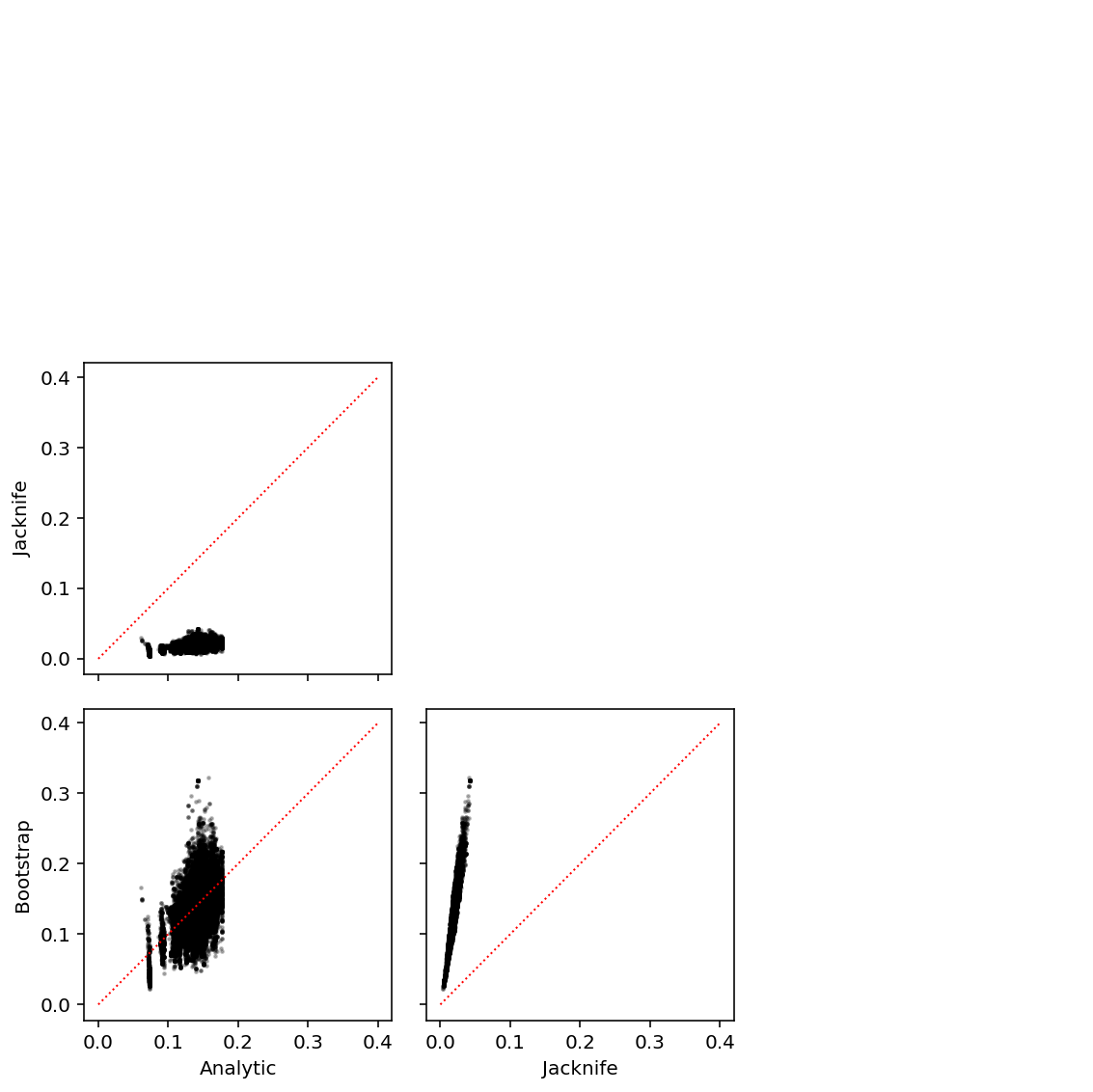
Compare standard error computations.

def jacknife(x, y):
  n = y.shape[0]
  # pandas is too clever here
  xty = x.values.T * y.values
  beta = xty.sum(axis=1) / n
  se = np.array([(n * beta - xty[:,i]) / (n - 1) for i in range(y.shape[0])]).std(axis=0)
  return beta, se

def bootstrap(x, y, b):
  n = y.shape[0]
  beta = x.values.T.dot(y.values) / n
  B = []
  for _ in range(b):
    index = np.random.choice(n, n, replace=True)
    B.append(x.iloc[index].values.T.dot(y.iloc[index]) / n)
  se = np.array(B).std(axis=0)
  return beta, se

def run_se_pass(vcf, pheno, header):
  np.random.seed(0)
  result = []
  for _, record in pheno.iterrows():
    x = read_dosage(vcf, record)
    if x is not None:
      x.index = header
      y = record
      x, y = x.align(y, axis='index', join='inner')
      y = y.astype(float)
      beta0, se0 = lm(x, y)
      _, se1 = jacknife(x, y)
      _, se2 = bootstrap(x, y, 100)
      result.append(pd.DataFrame({'gene': record.name, 'beta0': beta0, 'se0': se0, 'se1': se1, 'se2': se2}))
  return pd.concat(result)

res = run_se_pass(vcf, pheno.sample(n=100), header)

ticks = ['Analytic', 'Jacknife', 'Bootstrap']
plt.clf()
fig, ax = plt.subplots(3, 3, sharex=True, sharey=True)
fig.set_size_inches(8, 8)
for y in range(3):
  for x in range(3):
    if y <= x:
      ax[y, x].set_axis_off()
    else:
      ax[y, x].scatter(res['se{}'.format(x)], res['se{}'.format(y)], s=2, c='k', alpha=0.25)
      ax[y, x].plot([0, .4], [0, .4], c='r', ls=':', lw=1)
for y in range(3):
  ax[y, 0].set_ylabel(ticks[y])
for x in range(3):
  ax[-1, x].set_xlabel(ticks[x])
fig.tight_layout()

Downsample variants per gene like in Urbut et al 2016 to make the estimation problem easier.

def downsample(x, n):
  assert n >= 0
  if x.shape[0] >= n:
    return x.loc[np.random.choice(x.index, n, replace=False)]
  else:
    return x

def fit_ash(summary_stats):
  summary_stats = pd.read_table(summary_stats).groupby('gene').apply(downsample, n=10)
  return ashr.ash(summary_stats['beta'], summary_stats['se'], method='fdr', mixcompdist='normal')

Fit ash.

ash_results = {x: fit_ash('/scratch/midway2/aksarkar/singlecell/power/{}.txt.gz'.format(x))
               for x in ('log_phi', 'mean', 'bulk', 'resid', 'cv_resid')}

Serialize the results.

with open('/scratch/midway2/aksarkar/singlecell/power/ash-results.pkl', 'wb') as f:
  pickle.dump(ash_results, f)

Read the results.

with open('/scratch/midway2/aksarkar/singlecell/power/ash-results.pkl', 'rb') as f:
  ash_results = pickle.load(f)

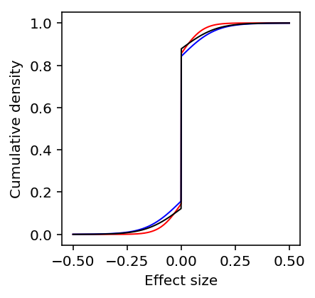
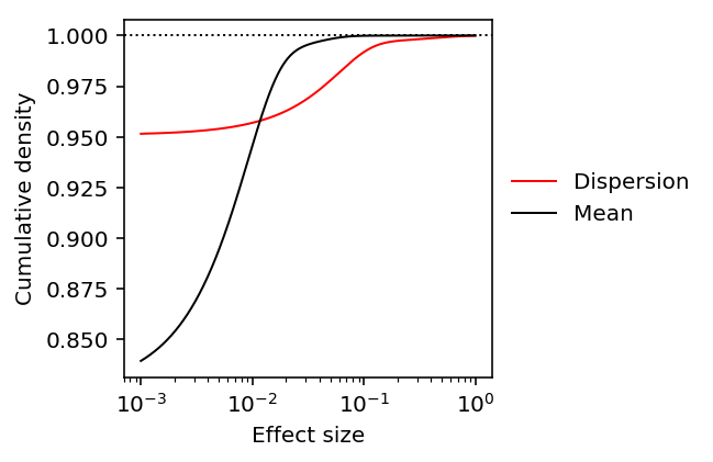
Plot the estimated distributions of effect sizes.

plt.clf()
plt.gcf().set_size_inches(3, 3)
grid = np.linspace(-.5, .5, num=1000)
for k, c, l in zip(ash_results, ['r', 'b', 'k'], ['Dispersion', 'Mean', 'Bulk']):
  y = np.array(ashr.cdf_ash(ash_results[k], grid).rx2('y')).ravel()
  plt.plot(grid, y, c=c, lw=1, label=l)
plt.xlabel('Effect size')
plt.ylabel('Cumulative density')

Text(0,0.5,'Cumulative density')

Run nominal passes on variance phenotypes.

sbatch --partition=broadwl -n1 -c28 --exclusive --job-name=nominal --out nominal.out --time=60:00
#!/bin/bash
source activate scqtl

Submitted batch job 47405002

Fit mash.

def fit_mash(df, g=None):
  betahat = df.iloc[:,:df.shape[1] // 2]
  se = df.iloc[:,df.shape[1] // 2:]
  data = mashr.mash_set_data(betahat, se)
  U = mashr.cov_canonical(data)
  if g is None:
    V = mashr.estimate_null_correlation(data)
    data = mashr.mash_set_data(betahat, se, V=V)
    return mashr.mash(data, U, verbose=True)
  else:
    return mashr.mash(data, verbose=True, fixg=True, g=g)

def train_test_split(betahat, se, train_subsample=10, test_thresh=9):
  df = pd.DataFrame(np.concatenate([betahat, se], axis=-1))
  training_set = df.groupby(stats[0]['gene']).apply(downsample, n=train_subsample)
  test_set = df[(np.square(betahat / se) > test_thresh).any(axis=1)]
  return training_set, test_set

def get_pairwise_sharing(stats):
  common = functools.reduce(lambda x, y: x.merge(y, on=['id', 'gene'], how='inner')[['id', 'gene']], stats)
  betahat = np.vstack([s.merge(common, on=['id', 'gene'], how='inner')['beta'] for s in stats]).T
  se = np.vstack([s.merge(common, on=['id', 'gene'], how='inner')['se'] for s in stats]).T
  training_set, test_set = train_test_split(betahat, se)
  mash_result0 = fit_mash(training_set)
  mash_result1 = fit_mash(test_set, g=mash_result0.rx2('fitted_g'))
  return np.array(mashr.get_pairwise_sharing(mash_result1))

stats = [pd.read_table('/scratch/midway2/aksarkar/singlecell/power/{}.txt.gz'.format(f)).rename(columns={'Unnamed: 0': 'id'})
         for f in ('bulk', 'log_mu','variance','fano','cv')]
# Bulk gene names need to be munged
stats[0]['gene'] = [x.split('.')[0] for x in stats[0]['gene']]
# CV effect sizes are expected to be anti-correlated to all others
stats[-1]['beta'] *= -1

res = get_pairwise_sharing(stats)

array([[1.        , 0.94283656, 0.94073996, 0.94026625, 0.94153343],
[0.94283656, 1.        , 0.99865977, 0.9935249 , 0.97356074],
[0.94073996, 0.99865977, 1.        , 0.9997103 , 0.9710184 ],
[0.94026625, 0.9935249 , 0.9997103 , 1.        , 0.97188708],
[0.94153343, 0.97356074, 0.9710184 , 0.97188708, 1.        ]])

pd.options.display.float_format = '{:.3g}'.format
ticks = ['Bulk', 'Abundance', 'Variance', 'Fano', 'CV']
pd.DataFrame(100 * res, columns=ticks, index=ticks)

Bulk  Abundance  Variance  Fano   CV
Bulk        100       94.3      94.1    94 94.2
Abundance  94.3        100      99.9  99.4 97.4
Variance   94.1       99.9       100   100 97.1
Fano         94       99.4       100   100 97.2
CV         94.2       97.4      97.1  97.2  100

Compare experimental variance to biological variance

Let \hat{\theta}_i be an estimate of some phenotype \(\theta_i\). Assume:

\[ \hat{\theta}_i = \theta_i + u_i \]

where \(u_i\) is a random effect capturing experimental noise, finite sampling variance, and estimator sampling variance.

Above, we estimated the scale of the finite sampling variance and estimator sampling variance. Here, we relate it to the genetic variance.

Extract the genotypes and UMI counts.

def parse_vcf_dosage(record):
  geno = [float(g) for g in record[9:]]
  return pd.Series(geno)

def extract_geno(qtls, dosages):
  header = pd.read_table(dosages, skiprows=2, nrows=1, header=0).columns[9:]
  genotypes = tabix.open(dosages)
  X = np.round(
    qtls
    .apply(lambda x: parse_vcf_dosage(next(genotypes.query(x['chr'], int(x['var_start']) - 1, int(x['var_start'])))), axis=1)
    .rename(columns={i: ind for i, ind in enumerate(header)}))
  return X

def extract_counts(qtls, counts):
  X = pd.concat(
    [chunk.align(qtls, axis='index', join='inner')[0]
     for chunk in pd.read_table(counts, index_col=0, chunksize=1000)])
  return X

def sample_counts(counts, n):
  X = pd.concat(
    [chunk.sample(n=n)
     for chunk in pd.read_table(counts, index_col=0, chunksize=1000)])
  return X

Read the data.

qtls = (pd.read_table('/project2/mstephens/aksarkar/projects/singlecell-qtl/data/scqtl-mapping/mean.txt.gz', sep=' ', index_col=0)
        .sample(n=200, random_state=1))
annotations = pd.read_table('/project2/mstephens/aksarkar/projects/singlecell-qtl/data/scqtl-annotation.txt')
keep_samples = pd.read_table('/project2/mstephens/aksarkar/projects/singlecell-qtl/data/quality-single-cells.txt', index_col=0, header=None)

Extract the subset we want.

counts = extract_counts(qtls, '/project2/mstephens/aksarkar/projects/singlecell-qtl/data/scqtl-counts.txt.gz')
annotations = annotations.loc[keep_samples.values.ravel()].reset_index(drop=True)
counts = counts.loc[:,keep_samples.values.ravel()]

Bootstrap the subset.

def bootstrap(counts, annotations):
  idx = np.hstack({k: np.random.choice(g, size=len(g))
                   for k, g in annotations.groupby('chip_id').groups.items()}.values())
  return counts.iloc[:,idx], annotations.iloc[idx]

Recover the derived mean and variance.

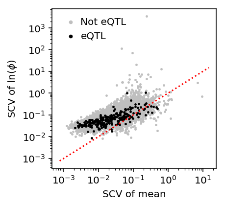
Compare the phenotypic variance of mean against dispersion. Use squared coefficient of variation to get dimensionless quantities.

scv = pd.Series(np.square(st.variation(mean_by_ind, axis=1)) / np.square(st.variation(log_phi, axis=1)))
scv.describe()

count    9957.000000
mean        0.388954
std         0.537197
min         0.000067
25%         0.164379
50%         0.267103
75%         0.459509
max        25.724706
dtype: float64

plt.clf()
plt.gcf().set_size_inches(3, 3)
plt.semilogx()
plt.semilogy()
all_qtls = (pd.read_table('/project2/mstephens/aksarkar/projects/singlecell-qtl/data/scqtl-mapping/mean.txt.gz', sep=' ', index_col=0)
            .sort_values('p_beta')
            .head(n=241))
plt.scatter(np.square(st.variation(mean_by_ind, axis=1)),
            np.square(st.variation(log_phi, axis=1)),
            s=2, c='.75', label='Not eQTL')
plt.scatter(np.square(st.variation(mean_by_ind.loc[all_qtls.index], axis=1)),
            np.square(st.variation(log_phi.loc[all_qtls.index], axis=1)),
            s=2, c='k', label='eQTL')
plt.plot(plt.xlim(), plt.xlim(), c='r', ls=':')
plt.legend(frameon=False, markerscale=2, handletextpad=0)
plt.xlabel('SCV of mean')
_ = plt.ylabel('SCV of $\ln(\phi)$')

Partition the sum of squares.

def ss(y):
  return np.square(y - y.mean()).sum()

def partition(x, y):
  total = ss(y)
  within = y.groupby(x.values).apply(ss).sum()
  between = total - within
  return total, between, within

geno = extract_geno(qtls, '/scratch/midway2/aksarkar/singlecell/scqtl-mapping/yri-120-dosages.vcf.gz')
geno = geno.loc[:,list(set(annotations['chip_id']))]
X, Y = geno.align(mean_by_ind, join='inner')
var_comps = pd.DataFrame([partition(X.loc[i], Y.loc[i]) for i in Y.index])
var_comps.index = X.index
var_comps.columns = ['total', 'between', 'within']

Look at the ANOVA for weak eQTLs.

var_comps.tail()

total       between        within
gene
ENSG00000163961  3.681769e-10  9.298483e-11  2.751920e-10
ENSG00000151806  1.530030e-10  5.271346e-11  1.002895e-10
ENSG00000116260  3.854593e-10  6.561917e-11  3.198401e-10
ENSG00000109775  3.234854e-10  1.171794e-10  2.063060e-10
ENSG00000164758  2.571498e-10  7.245402e-11  1.846958e-10

Compare against the estimated sampling variance from the simulation.

data[np.logical_and(data['num_samples'] == 95, data['num_mols'] == 114026)]['latent_mean_hat'].describe()

count    8.000000e+01
mean     9.264424e-09
std      2.667586e-08
min      1.169715e-11
25%      1.685388e-10
50%      9.926134e-10
75%      4.742833e-09
max      1.403023e-07
Name: latent_mean_hat, dtype: float64

Estimate bootstrap SEs on a GPU.

<<zinb-imports>>
<<tf-imports>>
import scipy.linalg as sl
import tabix

<<recode-impl>>
<<extract-impl>>
<<bootstrap-impl>>

<<read-qtls>>
<<extract-counts>>

log_mu = pd.read_table('/project2/mstephens/aksarkar/projects/singlecell-qtl/data/density-estimation/design1/zi2-log-mu.txt.gz', index_col=0, sep=' ').align(counts, axis='index', join='inner')[0]
log_phi = pd.read_table('/project2/mstephens/aksarkar/projects/singlecell-qtl/data/density-estimation/design1/zi2-log-phi.txt.gz', index_col=0, sep=' ').align(counts, axis='index', join='inner')[0]
logodds = pd.read_table('/project2/mstephens/aksarkar/projects/singlecell-qtl/data/density-estimation/design1/zi2-log-mu.txt.gz', index_col=0, sep=' ').align(counts, axis='index', join='inner')[0]

results = []
for trial in range(100):
  C, A = bootstrap(counts, annotations)
  onehot = recode(annotations, 'chip_id')
  chip = recode(annotations, 'experiment')
  chip -= chip.mean(axis=0)

  results.append(scqtl.tf.fit(
    umi=C.values.T.astype(np.float32),
    onehot=onehot.astype(np.float32),
    design=chip.astype(np.float32),
    size_factor=A['mol_hs'].astype(np.float32).values.reshape(-1, 1),
    warm_start=(log_mu.values.T.astype(np.float32), log_phi.values.T.astype(np.float32), logodds.values.T.astype(np.float32)),
    learning_rate=1e-3,
    max_epochs=30000,
    verbose=True,
  ))

estimates = {
  'mean': np.array([np.exp(r[0] - np.log1p(np.exp(r[2]))) for r in results]),
  'log_mean': np.array([r[0] - np.log1p(np.exp(r[2])) for r in results]),
  'disp': np.array([r[1] for r in results])
}

for k in estimates:
  (pd.DataFrame(estimates[k].var(axis=0).T, columns=sorted(set(annotations['chip_id'])), index=counts.index)
   .to_csv('/scratch/midway2/aksarkar/singlecell/power/{}-se.txt.gz'.format(k), sep='\t', compression='gzip'))

sbatch --partition=gpu2 --gres=gpu:1 --mem=16G --job-name=tf-zinb-se --out=tf-zinb-se.out
#!/bin/bash
source activate scqtl
python /project2/mstephens/aksarkar/projects/singlecell-qtl/code/tf-zinb-se.py

Submitted batch job 49257820

Read the results.

mean_sampling_var = pd.read_table('/scratch/midway2/aksarkar/singlecell/power/mean-se.txt.gz', index_col=0)
disp_sampling_var = pd.read_table('/scratch/midway2/aksarkar/singlecell/power/disp-se.txt.gz', index_col=0)

Estimate the reduction in effective PVE for eQTLs.

S, M = mean_sampling_var.align(mean_by_ind, join='inner', axis='index')
pd.DataFrame({'prop': S.mean(axis=1) / M.var(axis=1), 'factor': M.var(axis=1) / np.ma.masked_less((M.var(axis=1) - S.mean(axis=1)).values, 0)}).describe()

factor        prop
count  75.000000  100.000000
mean    3.365234    0.698366
std     4.746555    0.407146
min     1.109361    0.098580
25%     1.458076    0.380033
50%     2.043664    0.626091
75%     3.229525    0.978929
max    34.946118    2.004026

Estimate how many more cells would be required so the median factor is 1.1.

\[ (\sigma^2_y + \sigma^2_u) / \sigma^2_y \leq 1.1 \]

\[ \sigma^2_u \leq .1 \sigma^2 y \]

(S.mean(axis=1) / (.1 * np.ma.masked_less((M.var(axis=1) - S.mean(axis=1)).values, 0))).describe()

count     75.000000
mean      23.652338
std       47.465547
min        1.093611
25%        4.580756
50%       10.436642
75%       22.295255
max      339.461176
dtype: float64

(M.var(axis=1) / np.ma.masked_less((M.var(axis=1) - S.mean(axis=1) / 2.82).values, 0)).describe()

count    100.000000
mean       1.398247
std        0.388211
min        1.036224
25%        1.155754
50%        1.285377
75%        1.531795
max        3.455993
dtype: float64

Do the same for dQTLs.

S, M = disp_sampling_var.align(log_phi, join='inner', axis='index')
pd.DataFrame({'prop': S.mean(axis=1) / M.var(axis=1), 'factor': M.var(axis=1) / np.ma.masked_less((M.var(axis=1) - S.mean(axis=1)).values, 0)}).describe()

factor        prop
count  92.000000  100.000000
mean    2.346648    0.383063
std     3.382984    0.342855
min     1.041327    0.039686
25%     1.117332    0.108174
50%     1.281986    0.228490
75%     1.914243    0.636540
max    23.984483    1.541178

(S.mean(axis=1) / (.1 * np.ma.masked_less((M.var(axis=1) - S.mean(axis=1)).values, 0))).describe()

count     92.000000
mean      13.466479
std       33.829841
min        0.413266
25%        1.173316
50%        2.819856
75%        9.142426
max      229.844830
dtype: float64

Distribution of PVE

We can use shrunk marginal effect size estimates to bound the proportion of phenotypic variance explained. We claim:

\[ h^2 \geq \arg\max_j E[\beta_j \mid \hat\beta]^2 \]

Frequentist argument. If the maximizer \(j\) is causal, this is a lower bound on PVE because \(h^2 = \sum_k \beta_k^2\) and other variants \(k\) could be causal, and because the estimate is shrunk towards zero.

If it is not causal, then the true marginal effect size is \(\sum_i R_{ij} \beta_i\), where \(R_{ij} = \mathrm{Corr}(X_i, X_j)\). \(R_ij \leq 1\), so this is still a lower bound

Bayesian argument.

\[ h^2 \geq \beta_j^2 \text{ for all \(j\)} \]

\[ E[h^2 \mid \hat\beta] \geq E[\beta_j^2 \mid \hat\beta] \text{ for all \(j\)} \]

\[ E[h^2 \mid \hat\beta] \geq \arg\max_j E[\beta_j^2 \mid \hat\beta] \]

def get_pve(summary_stats, ash_result):
  res = ashr.ash(summary_stats['beta'], summary_stats['se'], fixg=True,
                 g=ash_result.rx2('fitted_g'))
  pve = np.square(pd.Series(np.square(ashr.get_psd(res)) + ashr.get_pm(res),
                            index=summary_stats['gene']))
  return pve.groupby(level=0).agg(max)

<<power-imports>>
<<downsample-impl>>
<<get-pve-impl>>
np.random.seed(0)
stats = {x: (pd.read_table('/scratch/midway2/aksarkar/singlecell/power/{}.txt.gz'.format(x))
             .groupby('gene')
             .agg(lambda x: x.loc[x['beta'].idxmax()])
             .reset_index())
         for x in ('log_phi', 'mean', 'bulk', 'resid', 'cv_resid')}
# Munge gene names in bulk summary statistics
stats['bulk']['gene'] = [x.split('.')[0] for x in stats['bulk']['gene']]
with open('/scratch/midway2/aksarkar/singlecell/power/ash-results.pkl', 'rb') as f:
  ash_results = pickle.load(f)
(pd.DataFrame({k: get_pve(v, ash_results[k]) for k, v in stats.items()})
 .to_csv('estimated-pve.txt.gz', sep='\t', compression='gzip'))

sbatch --partition=broadwl --time=10:00 --mem=4G -n1 -c28 --exclusive --job-name estimate-pve --out estimate-pve.out
#!/bin/bash
source activate scqtl
python /project2/mstephens/aksarkar/projects/singlecell-qtl/code/estimate-pve.py

Submitted batch job 47546035

Read the results.

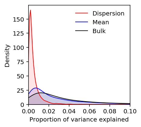
estimated_pve = pd.read_table('/scratch/midway2/aksarkar/singlecell/power/estimated-pve.txt.gz', index_col=0)
estimated_pve.columns = ['Bulk', 'CV residual', 'Dispersion', 'Mean', 'Residual']
estimated_pve = estimated_pve[['Dispersion', 'Mean', 'Bulk', 'Residual', 'CV residual']]

plt.clf()
plt.gcf().set_size_inches(3, 3)
M = 0.1
grid = np.linspace(0, M, 100)
for k, c in zip(estimated_pve, ['r', 'b', 'k']):
  f = st.gaussian_kde(estimated_pve[k].dropna())
  plt.plot(grid, f(grid), c=c, lw=1, label=k)
  plt.fill_between(grid, f(grid), color=c, alpha=0.1)
plt.legend(frameon=False)
plt.xlim(0, M)
plt.ylim(0, plt.ylim()[1])
plt.xlabel('Proportion of variance explained')
plt.ylabel('Density')

Text(0,0.5,'Density')

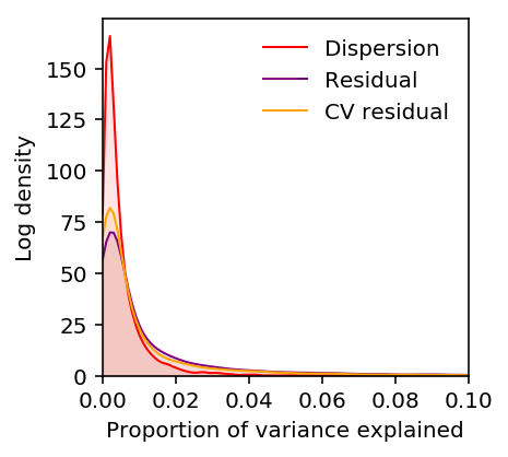
Plot the PVE of vQTLs/CV-QTLs after regressing out the mean.

plt.clf()
plt.gcf().set_size_inches(3, 3)
M = 0.1
grid = np.linspace(0, M, 100)
for k, c in zip(['Dispersion', 'Residual', 'CV residual'], ['r', 'purple', 'orange']):
  f = st.gaussian_kde(estimated_pve[k].dropna())
  plt.plot(grid, f(grid), c=c, lw=1, label=k)
  plt.fill_between(grid, f(grid), color=c, alpha=0.1)
plt.legend(frameon=False)
plt.xlim(0, M)
plt.ylim(0, plt.ylim()[1])
plt.xlabel('Proportion of variance explained')
plt.ylabel('Log density')

Text(0,0.5,'Log density')

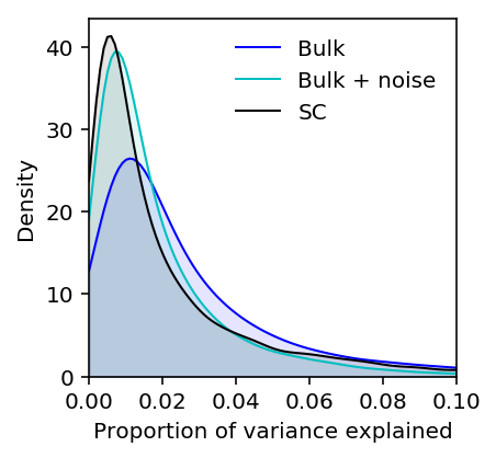
Plot the expected density of mean expression PVE assuming measurement noise from the simulation.

(estimated_pve['Mean'] / estimated_pve['Bulk']).describe()

count    8462.000000
mean        1.587743
std         3.075250
min         0.002746
25%         0.268501
50%         0.672904
75%         1.638187
max        62.349105
dtype: float64

plt.clf()
plt.gcf().set_size_inches(3, 3)
M = 0.1
grid = np.linspace(0, M, 100)
f0 = st.gaussian_kde(estimated_pve['Bulk'].dropna())
plt.plot(grid, f0(grid), c='b', lw=1, label='Bulk')
plt.fill_between(grid, f0(grid), color='b', alpha=0.1)

f1 = st.gaussian_kde(.67 * estimated_pve['Bulk'].dropna())
plt.plot(grid, f1(grid), c='c', lw=1, label='Bulk + noise')
plt.fill_between(grid, f1(grid), color='c', alpha=0.1)

f2 = st.gaussian_kde(estimated_pve['Mean'].dropna())
plt.plot(grid, f2(grid), c='k', lw=1, label='SC')
plt.fill_between(grid, f2(grid), color='k', alpha=0.1)

plt.legend(frameon=False)
plt.xlim(0, M)
plt.ylim(0, plt.ylim()[1])
plt.xlabel('Proportion of variance explained')
plt.ylabel('Density')

Text(0,0.5,'Density')

Estimate the proportion of large effect dQTLs.

f = st.gaussian_kde(estimated_pve['Dispersion'].dropna())
si.quad(f, .01, 1)

(0.06961646614211667, 4.412386762494795e-09)

Estimate the same for eQTLs.

f = st.gaussian_kde(estimated_pve['Bulk'].dropna())
si.quad(f, 0.01, 1)

(0.7296000671917134, 1.95708035203864e-12)

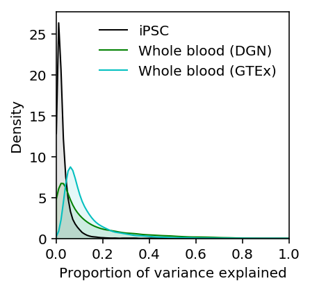
Compare the distribution of PVE for iPSCs against DGN whole blood (Wheeler et al 2016). The results are available on github.

import sqlite3
with sqlite3.connect('/project2/mstephens/aksarkar/.local/src/GenArchDB/genarch.db') as conn:
  dgn_pve = pd.read_sql('select * from results where tissue == "DGN-WB";', conn)
  gtex_pve = pd.read_sql('select * from results where tissue == "WholeBlood_TW" and pve != "NA";', conn)

plt.clf()
plt.gcf().set_size_inches(3, 3)
M = 0.1
grid = np.linspace(0, 1, 100)
f0 = st.gaussian_kde(estimated_pve['Bulk'].dropna())
plt.plot(grid, f0(grid), c='k', lw=1, label='iPSC')
plt.fill_between(grid, f0(grid), color='k', alpha=0.1)

f1 = st.gaussian_kde(dgn_pve['pve'].dropna())
plt.plot(grid, f1(grid), c='g', lw=1, label='Whole blood (DGN)')
plt.fill_between(grid, f1(grid), color='g', alpha=0.1)

f2 = st.gaussian_kde(gtex_pve['pve'].dropna())
plt.plot(grid, f2(grid), c='c', lw=1, label='Whole blood (GTEx)')
plt.fill_between(grid, f2(grid), color='c', alpha=0.1)

plt.legend(frameon=False)
plt.xlim(0, 1)
plt.ylim(0, plt.ylim()[1])
plt.xlabel('Proportion of variance explained')
plt.ylabel('Density')

Text(0,0.5,'Density')

Compute the expected power over the estimated distribution of PVE.

def average_power(g, f):
  x = g['pve']
  return si.trapz(g['power'] * f(x), x)

Estimate the distribution of effective PVE by correcting for the median reduction in PVE (at the current experiment size), and then assuming a large enough experiment to only reduce effective PVE by 10%..

f = st.gaussian_kde(.9 * estimated_pve['Bulk'].dropna())

Estimate the average power as a function of the number of individuals and number of causal variants.

(qtl_power.groupby(['num_individuals', 'num_causal']).apply(average_power, f=f)).reset_index()

num_individuals  num_causal         0
0               53        -1.0  0.067524
1               53         1.0  0.078898
2              100        -1.0  0.104900
3              100         1.0  0.114457
4              200        -1.0  0.152676
5              200         1.0  0.201122
6              300        -1.0  0.250451
7              300         1.0  0.280708
8              400        -1.0  0.276784
9              400         1.0  0.303322

Repeat the analysis for dQTLs.

(qtl_power.groupby(['num_individuals', 'num_causal']).apply(average_power, f=st.gaussian_kde(estimated_pve['Dispersion'].dropna() * .9 * 1.28))).reset_index()

num_individuals  num_causal         0
0               53        -1.0  0.008282
1               53         1.0  0.007657
2              100        -1.0  0.014693
3              100         1.0  0.015392
4              200        -1.0  0.016902
5              200         1.0  0.018266
6              300        -1.0  0.029801
7              300         1.0  0.031696
8              400        -1.0  0.030865
9              400         1.0  0.037992

Estimate the error variance

The single cell experiment size determines the standard error of the estimator, which can be thought of as measurement error.

\[ \hat\theta \sim N(\theta, \sigma^2) \]

This is the same as changing effective PVE:

\[ h^2_{\mathrm{eff}} = \frac{h^2}{1 + \sigma^2} \]

We estimate the standard error as a function of the experiment size from the simulation.

sim_results = pd.read_table('/scratch/midway2/aksarkar/singlecell/density-estimation/simulation.txt.gz', index_col=0)
sim_results['latent_mean'] = np.exp(sim_results['log_mu'] - np.log1p(np.exp(sim_results['logodds'])))
sim_results['latent_mean_hat'] = np.exp(sim_results['log_mu_hat'] - np.log1p(np.exp(sim_results['logodds_hat'])))
sim_results['latent_var'] = np.exp(2 * sim_results['log_mu'] + sim_results['log_phi'] - np.log1p(np.exp(sim_results['logodds']))) + np.exp(-np.log1p(np.exp(sim_results['logodds'])) - np.log1p(np.exp(-sim_results['logodds'])) + 2 * sim_results['log_mu'])
sim_results['latent_var_hat'] = np.exp(2 * sim_results['log_mu_hat'] + sim_results['log_phi_hat'] - np.log1p(np.exp(sim_results['logodds_hat']))) + np.exp(-np.log1p(np.exp(sim_results['logodds_hat'])) - np.log1p(np.exp(-sim_results['logodds_hat'])) + 2 * sim_results['log_mu_hat'])
mu_pass = sim_results['log_mu'] > -10
pi_pass = sim_results['logodds'] <= 0

Restrict the analysis to \(\ln\mu > -10, \mathrm{logit}(\pi) < 0\), because this is the part of the parameter space we can reliably estimate in.

data = sim_results[np.logical_and(mu_pass, pi_pass)].groupby(['num_samples', 'num_mols', 'latent_mean', 'latent_var'])[['latent_mean_hat', 'latent_var_hat']].agg(np.var).reset_index()

For \(x_1, \ldots, x_n \sim N(\mu, \sigma^2)\), we know:

\[ \bar{x} \sim N(\mu, \sigma^2 / n) \]

So a priori, we might expect the sampling variance of the single cell latent mean to decrease as \(1 / n\).

Similarly, we know:

\[ (n - 1)S^2 / \sigma^2 \sim \chi^2(n - 1) \]

Therefore,

\[ V[S^2] = 2 (n - 1) sigma^4 / (n - 1)^2 \]

And a priori, we might also expect the sampling variance of the single cell latent variance to decrease as \(1 / n\).

From the parametric simulation, we can estimate these relationships directly by fitting multiplicative models.

def mlm(x, y):
  x -= x.mean(axis=0)
  y -= y.mean()
  beta = np.linalg.pinv(x).dot(y)
  rss = np.square(y - x.dot(beta)).sum()
  sigma2 = rss / (y.shape[0] - 1)
  se = np.sqrt(sigma2 / np.einsum('ij,ij->j', x, x))
  return beta, se

def ci(beta, se):
  return np.array([beta + 1.96 * se, beta - 1.96 * se]).reshape(2, -1).T

ci(*mlm(np.log(data[['num_samples', 'num_mols', 'latent_mean', 'latent_var']]), np.log(data['latent_mean_hat'])))

array([[-0.9984868 , -1.03276978],
[-0.01299114, -0.08496202],
[-0.01580837, -0.07270787],
[ 1.01267559,  0.98504366]])

ci(*mlm(np.log(data[['num_samples', 'num_mols', 'latent_mean', 'latent_var']]), np.log(data['latent_var_hat'])))

array([[-0.94347526, -1.02803879],
[-0.07134441, -0.24887015],
[ 0.26219289,  0.12184272],
[ 1.92936491,  1.86120709]])

Analytic power calculation

We assume the generative process:

\[ y_i = x_i b + e_{\mathrm{resid}} \]

where \(y_i\) is the phenotype of individual \(i\), \(x_i\) is the genotype at the SNP of interest, and \(e_{\mathrm{resid}} \sim N(0, \sigma^2_r)\)

We observe \(y_i\) with error:

\[ \tilde{y}_i = y_i + e_{\mathrm{meas},i} \]

where \(e_{\mathrm{meas},i} \sim N(0, \sigma^2_m)\).

To perform QTL mapping, we fit a regression model:

\[ \tilde{y}_i = x_i \beta + \epsilon_i \]

where \(\epsilon_i \sim N(0, \sigma^2)\).

Assuming \(V[x] = 1\), we have:

\[\hat\beta \sim \mathcal{N}\left(b, \frac{\sigma^2_r + \sigma^2_m}{n}\right) \]

where \(n\) is the number of individuals.

Assume \(b = \lambda \sigma_r\), \(\lambda > 0\), and define \(\delta = \sigma^2_m / \sigma^2_r\) as the noise ratio. Then, the power at level \(\alpha\) is:

\[ \mathrm{Pow}(\lambda, n, \delta, \alpha) = p\left(\hat\beta > -\sigma_r \sqrt{\frac{1 + \delta}{n}} \Phi^{-1}\left(\frac{\alpha}{2}\right)\right) \]

\[ = \Phi\left(\Phi^{-1}\left(\frac{\alpha}{2}\right) + \lambda\sqrt{\frac{n}{1 + \delta}}\right) \]

where \(\Phi(\cdot)\) denotes the standard Gaussian CDF.

N = st.norm()

def power(lam, n, delta, alpha):
  return N.cdf(N.ppf(alpha / 2) + lam * np.sqrt(n / (1 + delta)))

Now, we need to answer the following questions:

What is the typical effect size?
What is the typical noise ratio of the current study?
How does the noise ratio vary with the number of cells and number of molecules?

Estimating the effect size distribution

To answer (1), we need to apply ash. To make effect sizes comparable between mean and dispersion, we need effect sizes in units of natural log fold change.

Compute effect sizes and standard errors.

<<power-imports>>
<<eqtl-sim-impl>>
<<write-pheno-def>>
<<nominal-pass-def>>

vcf = tabix.open('/scratch/midway2/aksarkar/singlecell/scqtl-mapping/yri-120-dosages.vcf.gz')
header = pd.read_table('/scratch/midway2/aksarkar/singlecell/scqtl-mapping/yri-120-dosages.vcf.gz', skiprows=2, nrows=1, header=0).columns[9:]

<<point-gamma-moments>>

<<get-gene-info>>
log_phi = (gene_info
           .apply(qtltools_format, axis=1)
           .merge(log_phi, left_index=True, right_index=True))
mean_by_ind = (gene_info
               .apply(qtltools_format, axis=1)
               .merge(np.log(mean_by_ind), left_index=True, right_index=True))

run_nominal_pass(vcf, log_phi, header, std=False).to_csv('disp.txt.gz', sep='\t', compression='gzip')
run_nominal_pass(vcf, mean_by_ind, header, std=False).to_csv('mean.txt.gz', sep='\t', compression='gzip')

sbatch --partition=broadwl -n1 -c28 --exclusive --job-name=nominal --out=nominal.out --time=60:00
#!/bin/bash
source activate scqtl
python /project2/mstephens/aksarkar/projects/singlecell-qtl/code/nominal-log-fc.py

Submitted batch job 55777035

Fit ash.

ash_results = {x: fit_ash('/scratch/midway2/aksarkar/singlecell/power/analytic/{}.txt.gz'.format(x))
               for x in ('mean', 'disp')}

Serialize the results.

with open('fold-change-ash-results.pkl', 'wb') as f:
  pickle.dump(ash_results, f)

Read the results.

with open('fold-change-ash-results.pkl', 'rb') as f:
  ash_results = pickle.load(f)

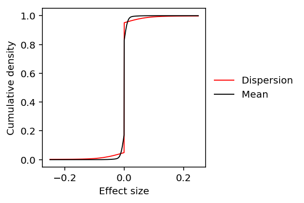
Look at the fitted \(g\).

plt.clf()
plt.gcf().set_size_inches(3, 3)
grid = np.linspace(-.25, .25, num=1000)
for k, c, l in zip(['disp', 'mean'], ['r', 'k'], ['Dispersion', 'Mean']):
  y = np.array(ashr.cdf_ash(ash_results[k], grid).rx2('y')).ravel()
  plt.plot(grid, y, c=c, lw=1, label=l)
plt.xlabel('Effect size')
plt.ylabel('Cumulative density')
plt.legend(frameon=False, loc='center left', bbox_to_anchor=(1, .5))

<matplotlib.legend.Legend at 0x7f483d809c88>

Look at the tail behavior of \(g\).

plt.clf()
plt.gcf().set_size_inches(3, 3)
plt.semilogx()
grid = np.logspace(-3, 0, num=1000)
for k, c, l in zip(['disp', 'mean'], ['r', 'k'], ['Dispersion', 'Mean']):
  y = np.array(ashr.cdf_ash(ash_results[k], grid).rx2('y')).ravel()
  plt.plot(grid, y, c=c, lw=1, label=l)
plt.axhline(y=1, c='k', lw=1, ls=':')
plt.xlabel('Effect size')
plt.ylabel('Cumulative density')
_ = plt.legend(frameon=False, loc='center left', bbox_to_anchor=(1, .5))

Get the effect size by percentile in the prior distribution.

def get_effect_size(ash_result, perc):
  grid = np.linspace(-.25, .25, 1000)
  return grid[np.where(np.array(ashr.cdf_ash(ash_result, grid).rx2('y')).ravel() > perc)][0]

mean_effect = get_effect_size(ash_results['mean'], .99)
mean_effect

0.022272272272272242

disp_effect = get_effect_size(ash_results['disp'], .99)
disp_effect

0.09034034034034033

Estimating the noise ratio

To answer (2), we need to estimate \(\sigma^2_m\) and \(\sigma^2_r\).

One complication is that we actually have \(e_{\mathrm{meas},i} \sim N(0, \sigma^2_{mi})\). We estimate \(\sigma^2_{mi}\) via non-parametric bootstrap for 200 randomly chosen genes.

sbatch --partition=gpu2 --gres=gpu:1 --time=12:00:00 --mem=16G --job-name=tf-zinb-se --out=tf-zinb-se.out
#!/bin/bash
source activate scqtl
python /project2/mstephens/aksarkar/projects/singlecell-qtl/code/tf-zinb-se.py

Submitted batch job 55782356

Read the results.

log_mean_sampling_var = pd.read_table('/scratch/midway2/aksarkar/singlecell/power/log_mean-se.txt.gz', index_col=0).filter(items=log_mu.columns, axis='columns')
disp_sampling_var = pd.read_table('/scratch/midway2/aksarkar/singlecell/power/disp-se.txt.gz', index_col=0).filter(items=log_mu.columns, axis='columns')

Naive approach

Assuming that \(\hat\sigma^2_{mi}\) is unbiased, \(\hat\sigma^2_r = \frac{1}{n - 1}\sum_i (\tilde{y}_i - \bar{y})^2 - \frac{1}{n}\sum_i \hat\sigma^2_{mi}\) is also unbiased (Buonaccorsi 2010, Eq. 10.1).

However, it can happen that \(\hat\sigma^2_r \leq 0\). We need the ratio \(\hat\sigma^2_m / \hat\sigma^2_r\) so this strategy may not work in general.

sigma2_m_mean_naive = log_mean_sampling_var.median(axis=1).median()
sigma2_r_mean_naive = (np.log(mean_by_ind).var(axis=1) - log_mean_sampling_var.median(axis=1)).median()
sigma2_m_mean_naive, sigma2_r_mean_naive

(0.012516903499999999, 0.005998688831110887)

sigma2_m_disp_naive = disp_sampling_var.median(axis=1).median()
sigma2_r_disp_naive = (log_phi.var(axis=1) - disp_sampling_var.median(axis=1)).median()
sigma2_m_disp_naive, sigma2_r_disp_naive

(3.0812910999999996, 0.6719321678084191)

Compare the phenotypic standard deviations.

np.sqrt(sigma2_r_disp_naive) / np.sqrt(sigma2_r_mean_naive)

10.583627575927432

Estimate the typical noise ratios.

delta_mean_naive = sigma2_m_mean_naive / sigma2_r_mean_naive
delta_disp_naive = sigma2_m_disp_naive / sigma2_r_disp_naive
delta_mean_naive, delta_disp_naive

(2.086606565602106, 4.585717498910597)

Full deconvolution approach

We can also use ash and vash (Lu and Stephens 2016) to solve the problem.

\[ \tilde{y}_i \mid y_i, \sigma^2_{mi} \sim \mathcal{N}(y_i, \sigma^2_{mi}) \]

We are primarily interested in the typical \(\sigma^2_r\) over all genes, rather than estimating \(y_i\) for each gene. Therefore, assume the observations \(\tilde{y}_i\) are centered to have mean 0 and jointly analyze observations across all genes, assuming a common prior.

\[ y_i \mid \hat\sigma^2_{mi} \sim g(\cdot) \]

where \(g\) is a unimodal mixture of uniforms.

Cordy and Thomas 1997 developed the same approach assuming \(\sigma^2_{mi} = \hat\sigma^2_{mi}\).

To estimate the typical \(\sigma^2_m\) over all genes, we could instead assume a hierarchical model on \(\hat\sigma^2_{mi}\).

\[ \hat\sigma^{2}_{mi} \mid \sigma^2_{mi}, \nu_i \sim \mathrm{Gamma}(\cdot) \]

where \(\nu_i\) denotes the degrees of freedom for observation \(i\).

\[ \sigma^{-2}_{mi} \sim h(\cdot) \]

where \(h\) is a unimodal mixture of inverse Gamma distributions.

Let \(\tilde\sigma^2_{mi} = 1 / E[\sigma^{-2}_{mi} \mid \cdot]\), and let \(\tilde{\nu}_i\) denote the posterior mean degrees of freedom. Then,

\[ \tilde{y}_i \mid y_i, \tilde\sigma^2_{mi}, \tilde{\nu}_i \sim t(y_i, \tilde\sigma^2_{mi}, \tilde{\nu}_i) \]

where \(t(\cdot)\) denotes the generalized \(t\) distribution.

Although it would be ideal to jointly estimate \(g\), \(h\), we can take a simpler approach:

Given \(\hat\sigma^2_{mi}, \nu_i\), use vash to estimate \(h\), \(\tilde\sigma^2_{mi}\), \(\tilde\nu_i\)
Given \(\tilde{y}_i\), \(\tilde\sigma^2_{mi}\), \(\tilde\nu_i\), use ash to estimate \(g\)

Then, the required variances are:

\[ \hat\sigma^2_r = V_g[y_i] \]

\[ \hat\sigma^2_m = 1 / E_h[\sigma^{-2}_{mi}] \]

def estimate_variances(y, se):
  y, se = y.align(se, join='inner')
  vash_res = vashr.vash(se.melt()['value'], df=y.shape[1] - 1, unimodal='precision')
  h = vash_res.rx2('fitted.g')
  pi = np.array(h.rx2('pi'))
  sigma2_m = pi.dot(ashr.comp_mean(h))
  # The observed df is equal for all observations, so the posterior mean df
  # will also be equal for all observations (Lu and Stephens 2016, eq. 13)
  df = 2 * np.array(vash_res.rx2('PosteriorShape')).dot(pi)[0]

  y = y.transform(lambda x: x - x.mean(), axis=1)
  lik = ashr.lik_t(df)
  res = ashr.ash(y.melt()['value'], vash_res.rx2('sd.post'), method='shrink', mixcompdist='uniform', lik=lik)
  g = res.rx2('fitted_g')
  sigma2_r = np.array(g.rx2('pi')).dot(np.square(np.array(g.rx2('b')) - np.array(g.rx2('a'))) / 12)
  return sigma2_m, sigma2_r

sigma2_m_mean_deconv, sigma2_r_mean_deconv = estimate_variances(np.log(mean_by_ind), np.sqrt(log_mean_sampling_var))
sigma2_m_mean_deconv, sigma2_r_mean_deconv

(0.030414726107298628, 0.008992095681497215)

sigma2_m_disp_deconv, sigma2_r_disp_deconv = estimate_variances(log_phi, np.sqrt(disp_sampling_var))
sigma2_m_disp_deconv, sigma2_r_disp_deconv

(2.1619294225792225, 1.805227380090225)

Serialize the results.

with open('deconvolution-results.pkl', 'wb') as f:
  pickle.dump((sigma2_m_mean_deconv, sigma2_r_mean_deconv, sigma2_m_disp_deconv, sigma2_r_disp_deconv), f)

Read the results.

with open('deconvolution-results.pkl', 'rb') as f:
  sigma2_m_mean_deconv, sigma2_r_mean_deconv, sigma2_m_disp_deconv, sigma2_r_disp_deconv = pickle.load(f)

Compare the phenotypic standard deviations.

np.sqrt(sigma2_r_disp_deconv) / np.sqrt(sigma2_r_mean_deconv)

14.16887915444257

Finally, get the typical noise ratios.

delta_mean_deconv = sigma2_m_mean_deconv / sigma2_r_mean_deconv
delta_disp_deconv = sigma2_m_disp_deconv / sigma2_r_disp_deconv
delta_mean_deconv, delta_disp_deconv

(3.3823846169566636, 1.1975939687282882)

Hybrid approach

In practice, the median of medians approach produces an acceptable estimate of the typical measurement error variance. However, the naive estimate of the residual variance is very different from the deconvolution estimate.

The results suggest that we could simplify the overall procedure by just applying ash as in Cordy and Thomas 1997.

def estimate_sigma2_r(y, se):
  y, se = y.align(se, join='inner')
  y = y.transform(lambda x: x - x.mean(), axis=1)
  res = ashr.ash(y.melt()['value'], se.melt()['value'], method='shrink', mixcompdist='uniform')
  g = res.rx2('fitted_g')
  sigma2_r = np.array(g.rx2('pi')).dot(np.square(np.array(g.rx2('b')) - np.array(g.rx2('a'))) / 12)
  return sigma2_r

sigma2_m_mean_hybrid = log_mean_sampling_var.median(axis=1).median()
sigma2_r_mean_hybrid = estimate_sigma2_r(np.log(mean_by_ind), np.sqrt(log_mean_sampling_var))
sigma2_m_mean_hybrid, sigma2_r_mean_hybrid

(0.012516903499999999, 0.009395909348799603)

sigma2_m_disp_hybrid = disp_sampling_var.median(axis=1).median()
sigma2_r_disp_hybrid = estimate_sigma2_r(log_phi, np.sqrt(disp_sampling_var))
sigma2_m_disp_hybrid, sigma2_r_disp_hybrid

(3.0812910999999996, 1.8152649700895214)

Compare the phenotypic standard deviations.

np.sqrt(sigma2_r_disp_hybrid) / np.sqrt(sigma2_r_mean_hybrid)

13.899545657433398

Finally, get the typical noise ratios.

delta_mean_hybrid = sigma2_m_mean_hybrid / sigma2_r_mean_hybrid
delta_disp_hybrid = sigma2_m_disp_hybrid / sigma2_r_disp_hybrid
delta_mean_hybrid, delta_disp_hybrid

(1.3321652045950323, 1.6974332401996624)

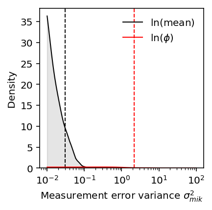
Comparison of the approaches

To understand why the results for the residual variance are different, first look at the distribution of measurement error variances. For reference, put the `vash` estimates on this plot.

plt.clf()
plt.gcf().set_size_inches(3, 3)
plt.semilogx()
grid = np.logspace(-2, 2, 100)

f = st.gaussian_kde(log_mean_sampling_var.values.ravel())
y = f(grid)
plt.plot(grid, y, lw=1, c='k', label=r'$\ln(\mathrm{mean})$')
plt.fill_between(grid, y, lw=1, color='k', alpha=0.1)
plt.axvline(x=sigma2_m_mean_deconv, lw=1, c='k', ls='--')

f = st.gaussian_kde(disp_sampling_var.values.ravel())
y = f(grid)
plt.plot(grid, y, lw=1, c='r', label=r'$\ln(\phi)$')
plt.fill_between(grid, y, lw=1, color='r', alpha=0.1)
plt.axvline(x=sigma2_m_disp_deconv, lw=1, c='r', ls='--')

plt.legend(frameon=False)

plt.ylim(0, plt.ylim()[1])
plt.xlabel(r'Measurement error variance $\sigma^2_{mik}$')
_ = plt.ylabel('Density')

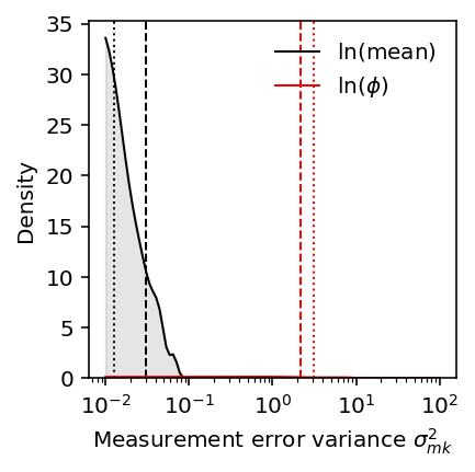
Then look at the distribution of estimated per-gene measurement error variances. For reference, put both the vash estimate and the naive estimate.

plt.clf()
plt.gcf().set_size_inches(3, 3)
plt.semilogx()
grid = np.logspace(-2, 2, 100)

f = st.gaussian_kde(log_mean_sampling_var.median(axis=1))
y = f(grid)
plt.plot(grid, y, lw=1, c='k', label='$\ln(\\mathrm{mean})$')
plt.fill_between(grid, y, lw=1, color='k', alpha=0.1)
plt.axvline(x=sigma2_m_mean_naive, lw=1, c='k', ls=':')
plt.axvline(x=sigma2_m_mean_deconv, lw=1, c='k', ls='--')

f = st.gaussian_kde(disp_sampling_var.median(axis=1))
y = f(grid)
plt.plot(grid, y, lw=1, c='r', label='$\ln(\phi)$')
plt.fill_between(grid, y, lw=1, color='r', alpha=0.1)
plt.axvline(x=sigma2_m_disp_naive, lw=1, c='r', ls=':')
plt.axvline(x=sigma2_m_disp_deconv, lw=1, c='r', ls='--')

plt.legend(frameon=False)

plt.ylim(0, plt.ylim()[1])
plt.xlabel(r'Measurement error variance $\sigma^2_{mk}$')
_ = plt.ylabel('Density')

Look at the distribution of naive residual variance estimates.

plt.clf()
plt.gcf().set_size_inches(3, 3)
plt.xscale('symlog', linthresh=1e-2)
grid = np.linspace(-10, 10, 100)

sigma2_rk_mean_naive = (np.log(mean_by_ind).var(axis=1) - log_mean_sampling_var.median(axis=1)).dropna()
f = st.gaussian_kde(sigma2_rk_mean_naive)
y = f(grid)
plt.plot(grid, y, lw=1, c='k', label='$\ln(\\mathrm{mean})$')
plt.fill_between(grid, y, lw=1, color='k', alpha=0.1)

sigma2_rk_disp_naive = (log_phi.var(axis=1) - disp_sampling_var.median(axis=1)).dropna()
f = st.gaussian_kde(sigma2_rk_disp_naive)
y = f(grid)
plt.plot(grid, y, lw=1, c='r', label='$\ln(\phi)$')
plt.fill_between(grid, y, lw=1, color='r', alpha=0.1)

plt.legend(frameon=False, loc='center left', bbox_to_anchor=(1, .5))

plt.xlabel(r'Naive residual variance $\sigma^2_{rk}$')
_ = plt.ylabel('Density')

The results suggest the fully naive version will not produce reasonable estimates of the typical residual variance.

Per-gene approach

The comparison above suggests that the noise ratio varies widely between genes. Therefore, instead of attempting to find a typical measurement error variance and a typical residual variance, we should keep the paired \(\sigma^2_{mk}, \sigma^2_{rk}\) and estimate the distribution of noise ratios.

def estimate_paired_variances(y, se):
  y, se = y.align(se, join='inner')
  sigma2_mk = np.square(se).median(axis=1)

  y = y.transform(lambda x: x - x.mean(), axis=1)
  res = ashr.ash(y.melt()['value'], se.melt()['value'], method='shrink', mixcompdist='uniform')
  ypost = pd.DataFrame(np.array(ashr.get_pm(res)).reshape(y.shape), index=y.index, columns=y.columns)
  sigma2_rk = ypost.var(axis=1)
  return sigma2_mk, sigma2_rk

Estimate the noise ratios for the mean.

sigma2_mk_mean_deconv, sigma2_rk_mean_deconv = estimate_paired_variances(np.log(mean_by_ind), np.sqrt(log_mean_sampling_var))
delta_mean = sigma2_mk_mean_deconv / sigma2_rk_mean_deconv

Estimate the noise ratios for the dispersion.

sigma2_mk_disp_deconv, sigma2_rk_disp_deconv = estimate_paired_variances(log_phi, np.sqrt(disp_sampling_var))
delta_disp = sigma2_mk_disp_deconv / sigma2_rk_disp_deconv

Plot the distribution of noise ratios.

f_mean = st.gaussian_kde(delta_mean)
f_disp = st.gaussian_kde(delta_disp)
grid = np.logspace(-3, 3, 100)
d_mean = f_mean(grid)
d_disp = f_disp(grid)

plt.clf()
plt.gcf().set_size_inches(3, 3)
plt.semilogx()

plt.plot(grid, d_mean, color='k', lw=1, label='$\ln(\mathrm{mean})$')
plt.fill_between(grid, d_mean, color='k', alpha=0.1)
plt.axvline(delta_mean.median(), c='k', ls='--', lw=1)

plt.plot(grid, d_disp, color='r', lw=1, label='$\ln(\phi)$')
plt.fill_between(grid, d_disp, color='r', alpha=0.1)
plt.axvline(delta_disp.median(), c='r', ls='--', lw=1)

plt.legend(frameon=False, loc='center left', bbox_to_anchor=(1, .5))
plt.ylim(0, plt.ylim()[1])
plt.xlabel('Noise ratio')
_ = plt.ylabel('Density')

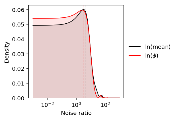
The distributions have large outliers, so take the median as the typical noise ratio across genes.

pd.DataFrame({'mean': delta_mean, 'disp': delta_disp}).describe()

disp        mean
count  200.000000  200.000000
mean     6.636096    8.827861
std     14.956849   12.738245
min      0.015321    0.118135
25%      0.530682    1.712591
50%      2.989148    4.177426
75%      6.443527    9.904404
max    147.443103   70.368543

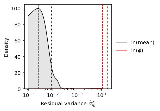
Plot the distribution of estimated residual variances. For reference, compare the median of the posterior means (dashed line) against the ash prior estimate (dotted line).

f_mean = st.gaussian_kde(sigma2_rk_mean_deconv)
f_disp = st.gaussian_kde(sigma2_rk_disp_deconv)
grid = np.logspace(-3, 0, 100)
d_mean = f_mean(grid)
d_disp = f_disp(grid)

plt.clf()
plt.gcf().set_size_inches(3, 3)
plt.semilogx()

plt.plot(grid, d_mean, color='k', lw=1, label='$\ln(\mathrm{mean})$')
plt.fill_between(grid, d_mean, color='k', alpha=0.1)
plt.axvline(sigma2_r_mean_deconv, c='k', ls=':', lw=1)
plt.axvline(sigma2_rk_mean_deconv.median(), c='k', ls='--', lw=1)

plt.plot(grid, d_disp, color='r', lw=1, label='$\ln(\phi)$')
plt.fill_between(grid, d_disp, color='r', alpha=0.1)
plt.axvline(sigma2_r_disp_deconv, c='r', ls=':', lw=1)
plt.axvline(sigma2_rk_disp_deconv.median(), c='r', ls='--', lw=1)

plt.legend(frameon=False, loc='center left', bbox_to_anchor=(1, .5))
plt.ylim(0, plt.ylim()[1])
plt.xlabel('Residual variance $\hat\sigma^2_{rk}$')
_ = plt.ylabel('Density')

Find the typical ratio between phenotypic standard deviations.

(np.sqrt(sigma2_rk_disp_deconv) / np.sqrt(sigma2_rk_mean_deconv)).median()

7.225724664347637

Dependence of measurement error on experiment size

To answer (3), we need to develop sampling theory of the ZINB distribution. As a first pass, assume that the sampling distributions of the mean and dispersion of the NB component remain unchanged.

Anscombe 1953 develops the sampling theory of the NB distribution, parameterized by mean \(m\) and size \(k\).

\[ \ln p(r) = r \ln (X) + k \ln(1 - X) + \ln \Gamma(k + r) - \ln \Gamma(k) - \ln \Gamma(r + 1) \]

where \(X = \frac{m}{m + k}\).

In our parameterization, we have \(m = R \mu\), \(k = \phi^{-1}\).

The MLE of \(m\) is \(\bar{r}\) where \(\bar{r}\) is the sample mean. Its sampling variance is:

\[ V[\hat{m}] = \frac{1}{N}\left(m + \frac{m^2}{k}\right) \]

which follows from properties of the sample mean.

The MLE of \(k\) is non-trivial, and its sampling variance is:

\[ V[\hat{k}] = \frac{2 k (k + 1)}{N X^2} \cdot \mathrm{const} \]

where \(N\) is the number of samples, and the constant does not depend on \(N\).

By the delta method,

\[ V[\ln(\hat\phi)] = V[-\ln(\hat{k})] = \frac{2 (k + 1)}{k N X^2} \cdot \mathrm{const} \]

where the constant remains unchanged.

Therefore, the sampling variance of \(\ln\phi\) also goes down linearly in the number of samples. Further, holding \(\sigma_r^2\) fixed, the noise ratio goes down linearly in the number of cells.

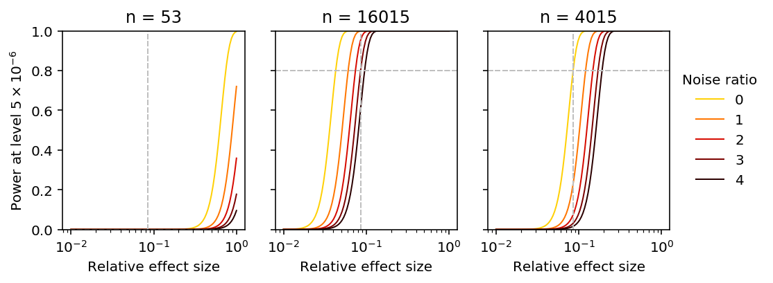
Power curves

Fixing \(\lambda, \alpha, \delta\), we can estimate the power achieved by the current study.

rel_effect = disp_effect / np.sqrt(sigma2_rk_disp_deconv.median())
alpha = 5e-6

pow_53 = power(rel_effect, 53, delta_disp.median(), alpha)
pow_53

1.0510141592463543e-05

We can solve analytically for the sample size \(n\) required to achieve 80% power, fixing the single cell experiment size (number of cell, number of molecules).

n_80 = int(np.ceil(np.square(N.ppf(.8) - N.ppf(alpha / 2)) * (1 + delta_disp.median()) / np.square(rel_effect)))
n_80

We can lower bound \(n\) by taking \(\delta \rightarrow 0\).

m_80 = int(np.ceil(np.square(N.ppf(.8) - N.ppf(alpha / 2)) * 1 / np.square(rel_effect)))
m_80

Now, plot the power function varying \(n, \delta\). Include reference points for the 99th percentile effect size relative to \(\sigma_r\), and the power achieved to detect effects of that size.

plt.clf()
fig, ax = plt.subplots(1, 3, sharey=True)
fig.set_size_inches(7, 3)
grid = np.logspace(-2, 0, 100)
for i, n in enumerate([53, n_80, m_80]):
  for ratio in np.linspace(0, 4, 5):
    scale = np.sqrt((1 + ratio) / n)
    power_ = N.cdf(N.ppf(alpha / 2) + grid / scale)
    color = colorcet.cm['fire_r']((ratio + .75) / 5)
    ax[i].set_xscale('log')
    ax[i].plot(grid, power_, lw=1, color=color, label='{:.2g}'.format(ratio))

    ax[i].axvline(x=rel_effect, c='.75', lw=1, ls='--')
    if i == 2:
      realized_scale = np.sqrt(1 / n)
    else:
      realized_scale = np.sqrt((1 + delta_disp.median()) / n)
    realized_power = N.cdf(N.ppf(alpha / 2) + rel_effect / realized_scale)
    ax[i].axhline(y=realized_power, c='.75', lw=1, ls='--')

    ax[i].set_ylim(0, 1)
    ax[i].set_title('n = {}'.format(n))
    ax[i].set_xlabel('Relative effect size')
ax[-1].legend(title='Noise ratio', frameon=False, bbox_to_anchor=(1, .5), loc='center left')
_ = ax[0].set_ylabel(r'Power at level $5 \times 10^{-6}$')
fig.tight_layout()