QTL mapping pipeline
Introduction
We take a modular approach to call QTLs:
- Estimate a mean and a dispersion for each individual
- Treat the mean/dispersion as continuous phenotypes and perform QTL mapping
Here, we solve (2).
- We reproduce eQTLs called on the bulk RNA-Seq
- We call mean/variance/CV/Fano QTLs using ZINB parameters
- We call QTLs using counts and log CPM
- We explain away variance QTLs
- We test replication/overlap between different QTL calls
Implementation
def cpm(x):
  return pd.DataFrame(pandas2ri.ri2py(edger.cpm(numpy2ri(x.values), log=True)),
                      columns=x.columns,
                      index=x.index)

def qqnorm(x):
  """Wrap around R qqnorm"""
  return np.asarray(rpy2.robjects.r['qqnorm'](numpy2ri(x))[0])

def bh(x):
  """Wrap around p.adjust(..., method='fdr')"""
  return np.asarray(rpy2.robjects.r['p.adjust'](numpy2ri(x), method='fdr'))
gene_info = (pd.read_table('/project2/mstephens/aksarkar/projects/singlecell-qtl/data/scqtl-genes.txt.gz')
             .set_index('gene')
             .query('source == "H. sapiens"')
             .query('chr != "hsX"')
             .query('chr != "hsY"')
             .query('chr != "hsMT"'))
with sqlite3.connect('/project2/mstephens/aksarkar/projects/singlecell-qtl/browser/browser.db') as conn:
  gene_info.to_sql('gene_info', conn, index=True, if_exists='replace')
def qtltools_format(row, prefix='chr'):
  row['#Chr'] = '{}{}'.format(prefix, row['chr'][2:])
  row['gid'] = row.name
  row['pid'] = row.name
  # Important: qtltools expects TSS start/end
  if row['strand'] == '+':
    row['end'] = row['start']
  else:
    row['start'] = row['end']
  return row.loc[['#Chr', 'start', 'end', 'pid', 'gid', 'strand']]

def write_pheno_file(pheno, gene_info, output_file, holdout=True, **kwargs):
  if holdout:
    genes = gene_info.loc[gene_info.apply(lambda x: bool(int(x['chr'][2:]) % 2), axis=1)]
  else:
    genes = gene_info
  (genes
   .apply(qtltools_format, **kwargs, axis=1)
   .merge(pheno, left_index=True, right_index=True)
   .to_csv(output_file,
           sep='\t',
           header=True,
           index=False,
           index_label=False))
export input=$input
sbatch --partition=$partition --wait
#!/bin/bash
module load bedtools
bedtools sort -header -i $input | bgzip >$input.gz
tabix -f -p bed $input.gz
export pheno=$pheno
export geno=$geno
export op=$op
sbatch --partition=$partition -a 1-100 -J $pheno-qtl --wait
#!/bin/bash
source activate scqtl
qtltools cis --vcf $geno --bed $pheno.bed.gz $op --chunk $SLURM_ARRAY_TASK_ID 100 --out $pheno-qtl.$SLURM_ARRAY_TASK_ID.txt --seed 0
def _read_helper(pheno, columns):
  file_names = ['{}-qtl.{}.txt'.format(pheno, i) for i in range(1, 101)]
  res = (pd.concat([pd.read_table(f, header=None, sep=' ')
                     for f in file_names if os.path.exists(f) and
                     os.path.getsize(f) > 0])
          .rename(columns={i: x for i, x in enumerate(columns)})
          .dropna()
          .sort_values('p_beta'))
  res['p_adjust'] = bh(res['p_beta'])
  res['fdr_pass'] = res['p_adjust'] < 0.1
  return res


def read_fastqtl_output(pheno):
  columns = ['gene', 'num_snps', 'a', 'b', 'dummy', 'id',
             'distance', 'p', 'beta', 'p_empirical', 'p_beta']
  res = _read_helper(pheno, columns)
  # Drop the gene version number
  res['gene'] = res['gene'].apply(lambda x: x.split('.')[0])
  res['chr'] = res['id'].apply(lambda x: x.split('.')[1])
  res['pos'] = res['id'].apply(lambda x: x.split('.')[2])
  res['id'] = res['id'].apply(lambda x: x.split('.')[0])
  return res

def read_qtltools_output(pheno):
  columns = ['gene', 'chr', 'start', 'end', 'strand', 'num_vars',
             'distance', 'id', 'var_chr', 'var_start', 'var_end', 'df',
             'dummy', 'a', 'b', 'p_nominal', 'beta', 'p_empirical', 'p_beta']
  res = _read_helper(pheno, columns)
  res['chr'] = res['var_chr']
  res['pos'] = res['var_start']
  res['id'] = res['id'].apply(lambda x: x.split('.')[0])
  return res

def read_nominal_pass(f):
  isf = st.chi2(1).isf
  result = pd.read_table(f, sep=' ', header=None)
  result.columns = ['gene', 'chr', 'start', 'end', 'strand', 'n', 'distance', 'id', 'var_chr', 'var_start', 'var_end', 'p_nominal', 'beta', 'top']
  result['z'] = np.sign(result['beta']) * np.sqrt(isf(result['p_nominal']))
  return result
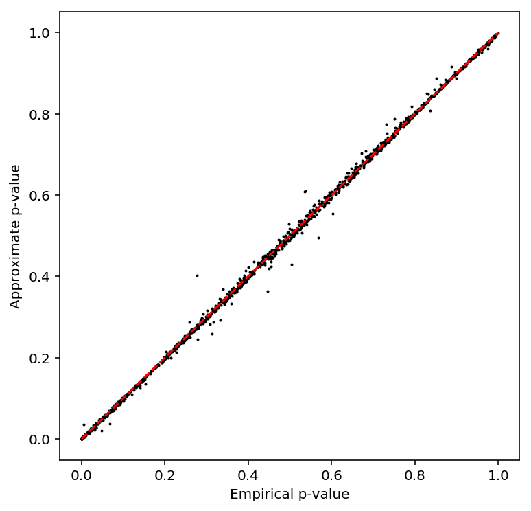
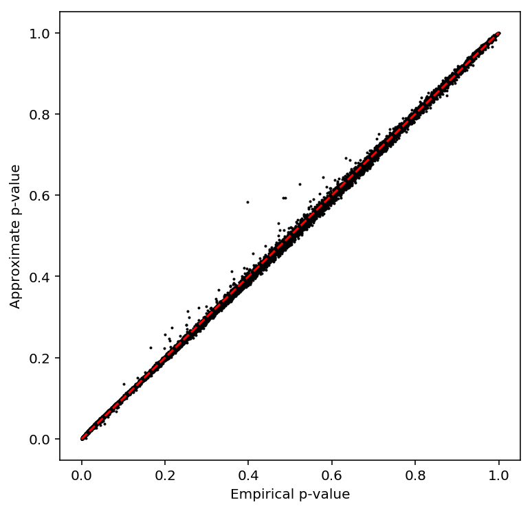
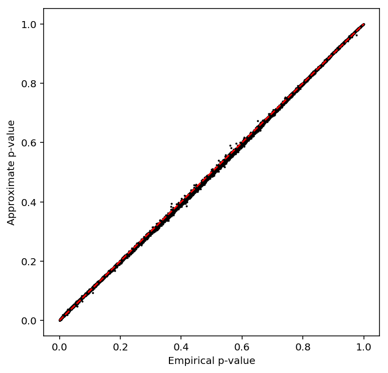
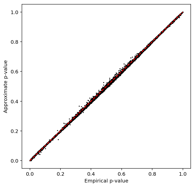
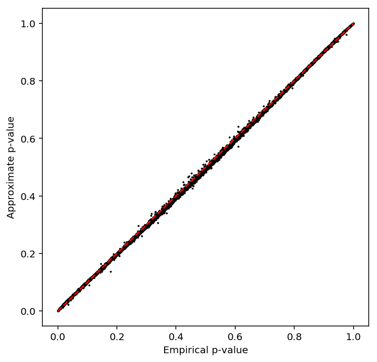
def plot_approx_permutation(df):
  plt.clf()
  plt.gcf().set_size_inches(6, 6)
  plt.scatter(df['p_empirical'], df['p_beta'], s=1, c='k')
  plt.plot([0, 1], [0, 1], c='r', ls='--')
  plt.xlabel('Empirical p-value')
  plt.ylabel('Approximate p-value')
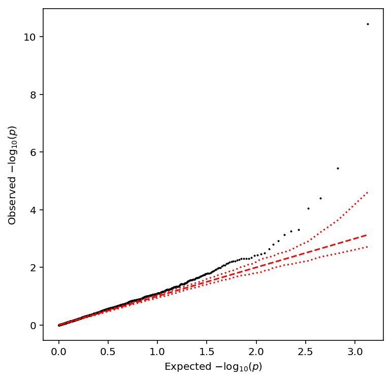
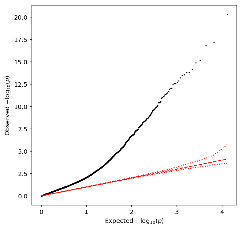
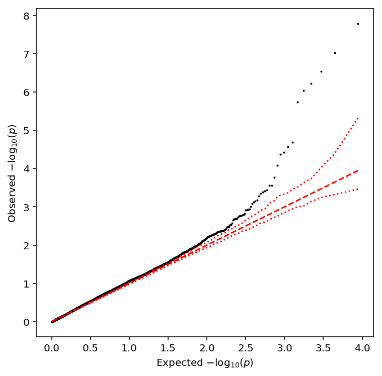
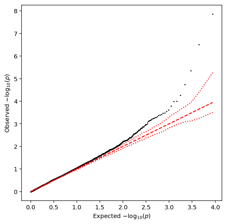
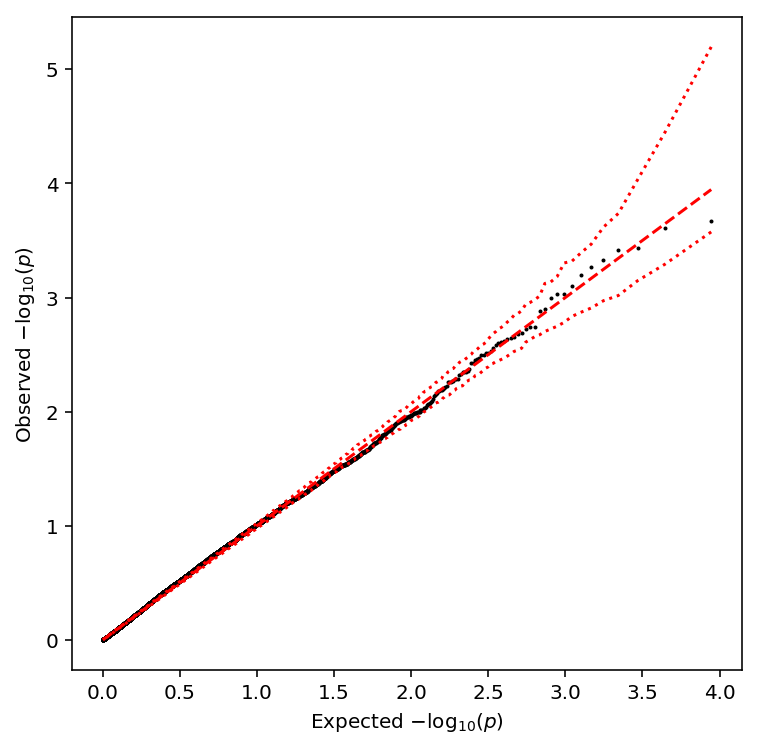
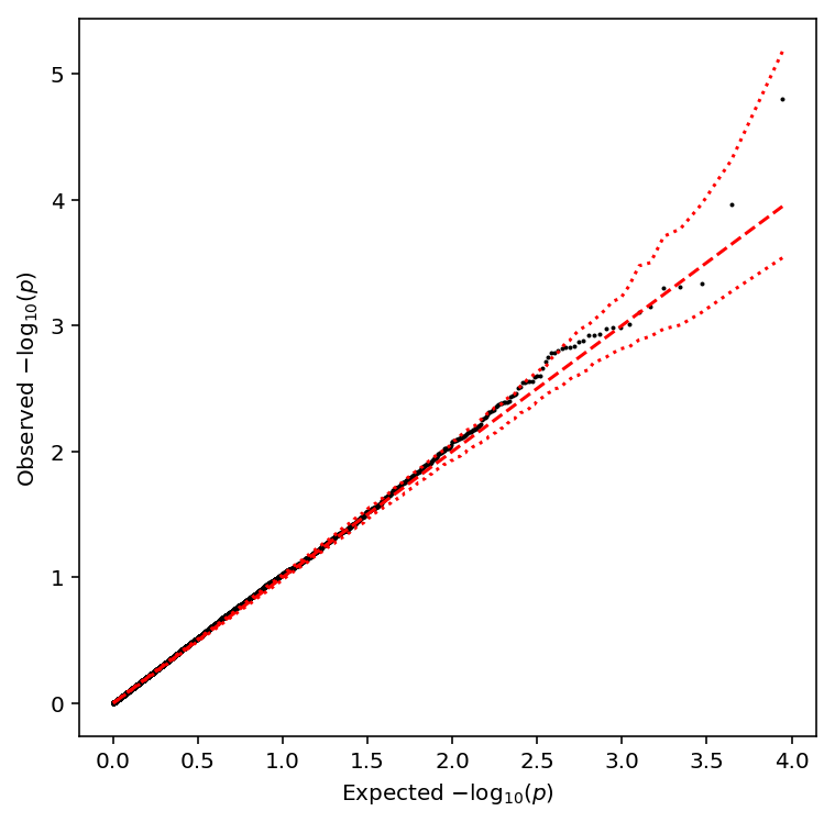
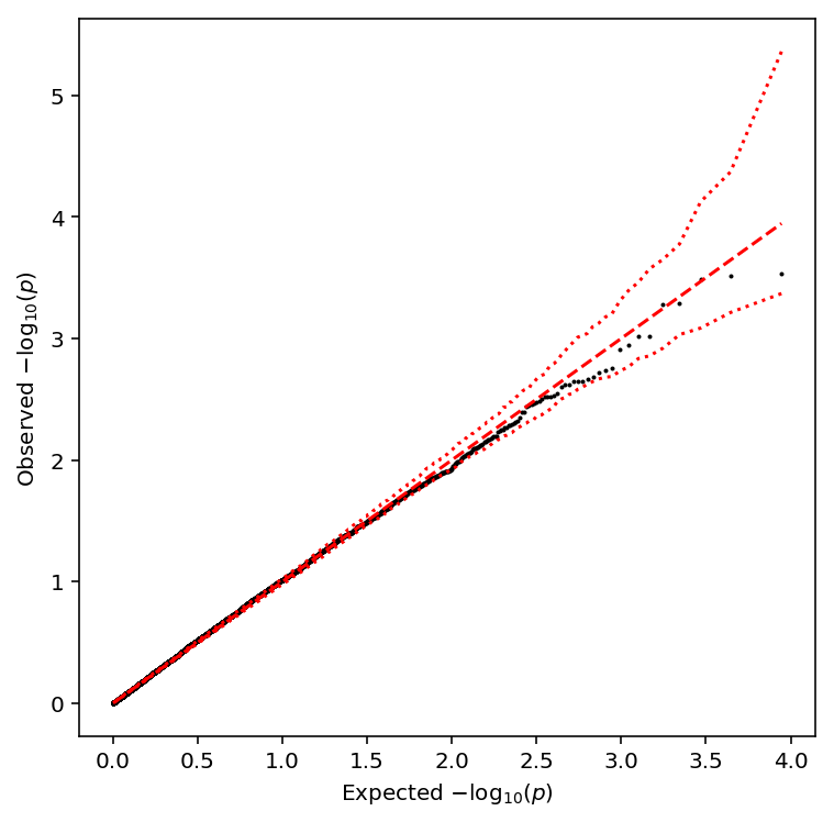
def qqplot(qtls):
  N = qtls.shape[0]
  # 95% bootstrap CI
  ci = -np.log10(np.percentile(np.sort(np.random.uniform(size=(100, N)), axis=1), [5, 95], axis=0))

  grid = -np.log10(np.arange(1, 1 + N) / N)
  plt.clf()
  plt.gcf().set_size_inches(6, 6)
  plt.scatter(grid, -np.log10(qtls['p_beta']), s=1, c='k')
  plt.plot([0, np.log10(qtls.shape[0])], [0, np.log10(qtls.shape[0])], c='r', ls='--')
  plt.plot(grid, ci[0], c='r', ls=':')
  plt.plot(grid, ci[1], c='r', ls=':')
  plt.xlabel('Expected $-\log_{10}(p)$')
  _ = plt.ylabel('Observed $-\log_{10}(p)$')
def parse_vcf_dosage(record):
  geno = [float(g) for g in record[9:]]
  return pd.Series(geno)

def extract_qtl_gene_pair(qtl_gene_df, pheno_df, dosages):
  """Return aligned genotype and phenotype matrix for each QTL-gene pair in qtl_gene_df"""
  common_phenos, common_qtls = pheno_df.align(qtl_gene_df.set_index('gene'), join='inner', axis=0)
  # Important: assume individual IDs are prefixed by "NA". This isn't true in
  # the original VCF
  header = pd.read_table(dosages, skiprows=2, nrows=1, header=0).columns[9:]
  genotypes = tabix.open(dosages)
  X, Y = (common_qtls
          .apply(lambda x: parse_vcf_dosage(next(genotypes.query(x['chr'], int(x['var_start']) - 1, int(x['var_start'])))), axis=1)
          .rename(columns={i: ind for i, ind in enumerate(header)})
          .align(common_phenos, join='inner', axis=None))
  return X, Y

def replication_tests(X, Y, C=None):
  """Return a DataFrame containing replication p-values

  X - centered dosage matrix (num_genes, num_individuals)
  Y - phenotype matrix (num_genes, num_individuals)
  C - confounder matrix (num_confounders, num_individuals)

  """
  p, n = X.shape
  assert Y.shape == (p, n)
  if C is not None:
    assert C.shape[1] == n
    C = np.array(C).T
    C = C - C.mean(axis=0)
    # Construct the annihilator matrix I - X X^+
    M = np.eye(n) - C.dot(np.linalg.pinv(C))
  result = []
  _sf = st.chi2(1).sf
  for (_, x), (name, y) in zip(X.iterrows(), Y.iterrows()):
    if np.isclose(x.std(), 0):
      print('Skipping {}'.format(name))
      continue
    x = x.values.copy().reshape(-1, 1)
    x -= x.mean()
    y = y.values.copy().ravel()
    y -= y.mean()
    if C is not None:
      y = M.dot(y)
      y -= y.mean()
    beta, rss, *_ = np.linalg.lstsq(x, y, rcond=-1)
    sigma2 = rss / y.shape[0]
    se = sigma2 / x.T.dot(x).ravel()
    pval = _sf(np.square(beta / se))
    result.append({'gene': name, 'beta': beta[0], 'se': se[0], 'p': pval.ravel()[0]})
  return pd.DataFrame.from_dict(result)

def pairwise_replication(qtls, phenos, ticks, covars=None):
  if covars is not None:
    assert len(covars) == len(phenos)
  assert len(phenos) == len(ticks)
  repl_rate = np.ones((len(phenos), len(phenos)))
  for i, ki in enumerate(phenos):
    for j, kj in enumerate(phenos):
      if i == j:
        continue
      q, p = qtls[ki][0], qtls[kj][1]
      X, Y = extract_qtl_gene_pair(q[q['fdr_pass']], p,
                                   dosages='/scratch/midway2/aksarkar/singlecell/scqtl-mapping/yri-120-dosages.vcf.gz')
      if X.empty:
        continue
      if covars is not None and covars[j] is not None:
        C = covars[j].align(X, axis='columns', join='inner')[0]
      else:
        C = None
      replication = q.merge(
        replication_tests(X, Y, C),
        on='gene',
        suffixes=['_1', '_2'])[['gene', 'id', 'beta_1', 'beta_2', 'p']]
      replication['fdr_pass'] = bh(replication['p']) < .1
      replication['replicated'] = replication.apply(lambda x: x['fdr_pass'] and x['beta_1'] * x['beta_2'] > 0, axis=1)
      repl_rate[i, j] = replication['replicated'].sum() / replication.shape[0]
  return pd.DataFrame(100 * repl_rate, columns=ticks, index=ticks)
def bootstrap_se(X, Y, C=None, num_bootstraps=100, seed=0):
  np.random.seed(seed)
  beta = {}
  for i in range(num_bootstraps):
    b = np.random.choice(X.shape[1], size=X.shape[1], replace=True)
    if C is not None:
      beta[i] = replication_tests(X.iloc[:,b], Y.iloc[:,b], C.iloc[:,b]).set_index('gene')['beta']
    else:
      beta[i] = replication_tests(X.iloc[:,b], Y.iloc[:,b]).set_index('gene')['beta']
  return pd.DataFrame.from_dict(beta).agg(np.std, axis=1)
def _fit_lm(x, y):
  n, p = x.shape
  assert y.shape == (n, 1)
  y -= y.mean()
  x -= x.mean(axis=0)
  beta = x.T.dot(y) / np.var(x, axis=0).values.reshape(-1, 1)
  return beta

def estimate_beta_se(genes, dosages, gene_info, covars=None, window=100000, n_bootstrap=100, seed=0):
  """Estimate beta via OLS and SE via bootstrap

  genes - dataframe (num_genes, num_individuals)
  dosages - VCF file name
  gene_info - dataframe (see read_gene_info)
  covars - dataframe (num_covars, num_individuals)

  """
  with gzip.open(dosages, 'rt') as f:
    for line in f:
      if line.startswith('#CHROM'):
        header = line.split()[9:]
        break
  dosages = tabix.open(dosages)
  if covars is not None:
    covars, genes = covars.align(genes, axis='columns', join='inner')
    _, n = covars.shape
    covars = covars.values.T
    M = np.eye(n) - covars.dot(np.linalg.pinv(covars))
  result = []
  for gene, Y in genes.iterrows():
    if gene in gene_info.index:
      record = gene_info.loc[gene]
      if record['strand'] == '+':
        X = dosages.query('chr{}'.format(record['chr'][2:]), record['start'] - window, record['start'] + window)
      else:
        X = dosages.query('chr{}'.format(record['chr'][2:]), record['end'] - window, record['end'] + window)
      X = list(X)
      meta = [row[2] for row in X]
      X = pd.DataFrame([parse_vcf_dosage(row) for row in X])
      X.index = meta
      X.columns = header
      X, Y = X.align(Y, axis='columns', join='inner')
      if covars is not None:
        Y = M.dot(Y - Y.mean())
      X = X.transform(lambda x: x - x.mean(), axis=1)

      beta = [_fit_lm(X.T, Y.reshape(-1, 1))]
      np.random.seed(seed)
      for _ in range(n_bootstrap):
        B = np.random.choice(n, size=n, replace=True)
        beta.append(_fit_lm(X.iloc[:,B].T, Y[B].reshape(-1, 1)))
      result.append(pd.DataFrame({'gene': gene, 'snp': meta, 'beta': beta[0].values.ravel(), 'se': np.std(np.ma.masked_invalid(np.hstack(beta[1:])), axis=1)}))
  return pd.concat(result)
Preliminaries
Test validity of approximate permutation test
qtltools tries to calibrate false discovery rates using the following
procedure:
- For each gene, permute the genotype data to estimate the null distribution of the p-values
- Fit a beta distribution to the permuted p-values via ML
- Compute the lower tail probability of the observed p-value, assuming it was generated from the fitted beta distribution
- Apply FDR correction on the set of lower tail probabilities (across all genes)
Test whether the beta approximation is appropriate for our sample size by subsetting GEUVADIS. Take all genes on chromosome 1.
geuvadis = []
for chunk in pd.read_table('/project/compbio/geuvadis/analysis_results/GD462.GeneQuantRPKM.50FN.samplename.resk10.txt.gz', chunksize=100):
  geuvadis.append(chunk.query('Chr == "1"'))
geuvadis = pd.concat(geuvadis)
geuvadis = geuvadis.set_index(geuvadis['Gene_Symbol'].apply(lambda x: x.split('.')[0]))
First, replicate the result in Delaneau et al 2017 by using all 462 individuals from GEUVADIS.
pd.Series(geuvadis.columns).sort_values().to_csv('/scratch/midway2/aksarkar/singlecell/geuvadis/geuvadis-subset.txt', header=None, index=None)
Write out the phenotype file for qtltools. Important: GEUVADIS VCFs code
chromosome without chr.
write_pheno_file(geuvadis, gene_info, '/scratch/midway2/aksarkar/singlecell/geuvadis/test.bed', prefix='')
Index the phenotype file. Important: # sorts before c, but after 1.
Submitted batch job 44542169
Perform SNP QC in plink.
sbatch --partition=broadwl --mem=2G --wait
#!/bin/bash
plink --memory 2000 --geno 0.01 --maf 0.05 --keep-fam /scratch/midway2/aksarkar/singlecell/geuvadis-subset.txt --vcf /project/compbio/geuvadis/genotypes/GEUVADIS.chr1.PH1PH2_465.IMPFRQFILT_BIALLELIC_PH.annotv2.genotypes.vcf.gz --recode vcf-iid --out geuvadis-chr1
bgzip -f geuvadis-chr1.vcf
tabix -f -p vcf geuvadis-chr1.vcf.gz
Submitted batch job 44541229
Run qtltools.
Submitted batch job 44685856
Read the results.
geuvadis_qtls = read_qtltools_output('geuvadis/test')
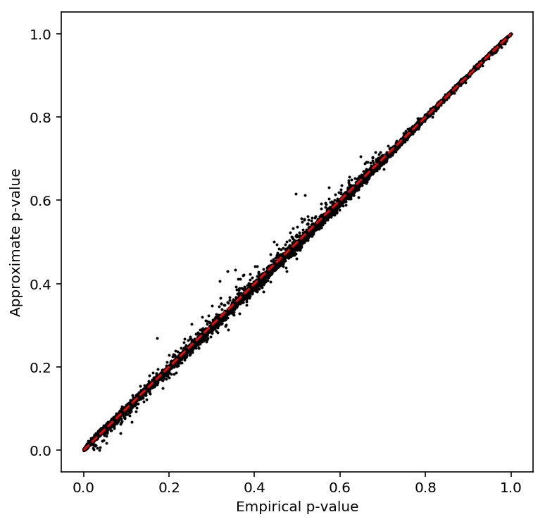
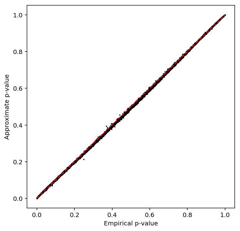
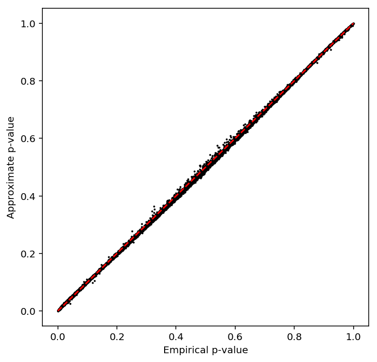
Check the beta approximation to the permutation p-values.
plot_approx_permutation(geuvadis_qtls)

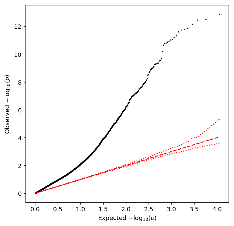
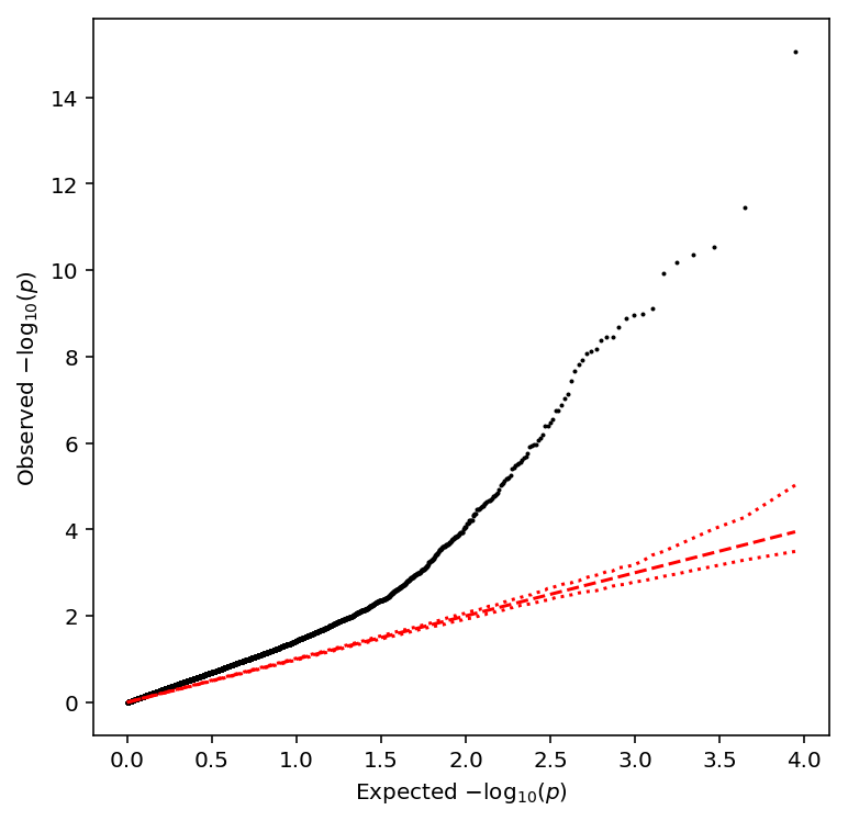
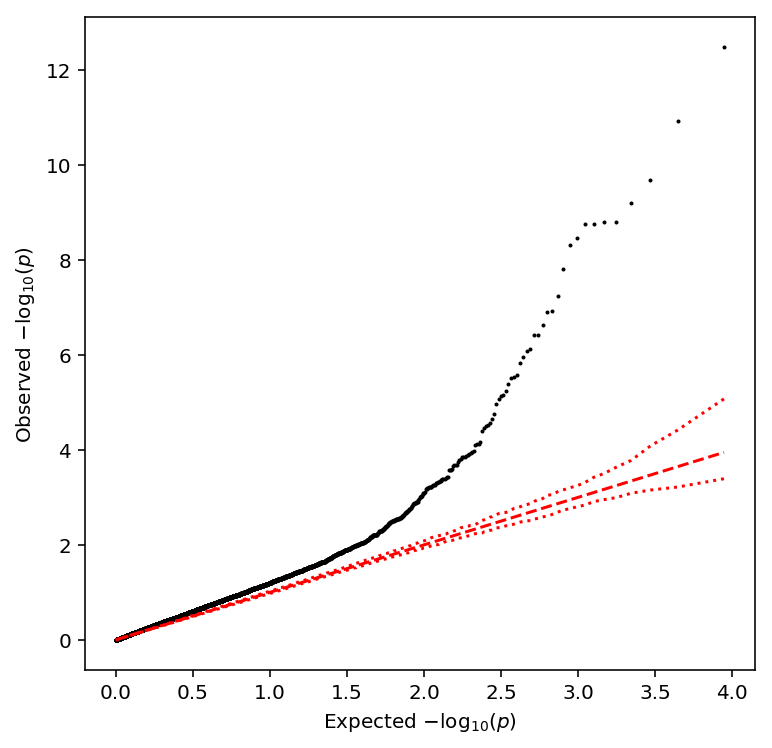
Plot the QQ plot
qqplot(geuvadis_qtls)
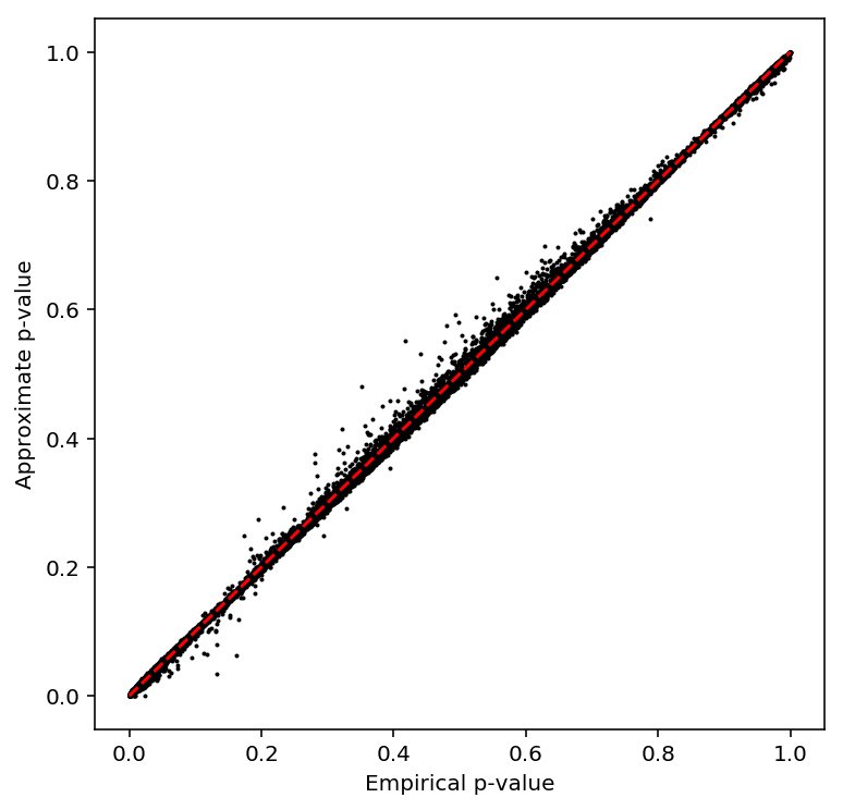
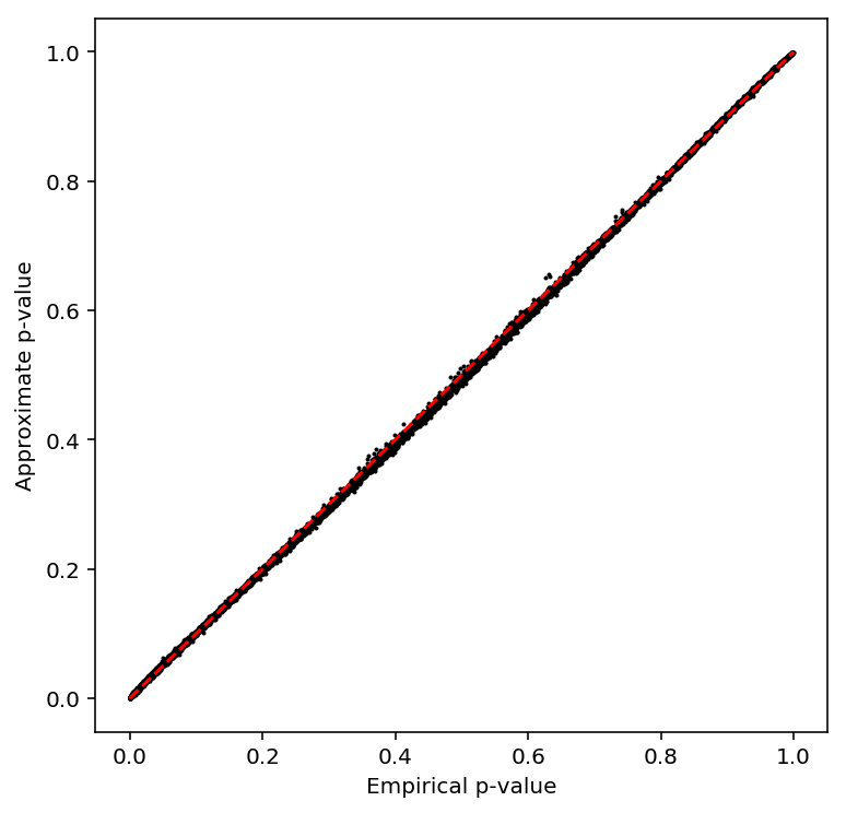
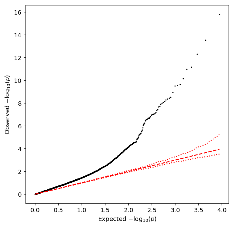
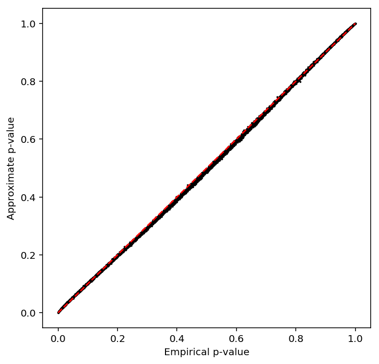
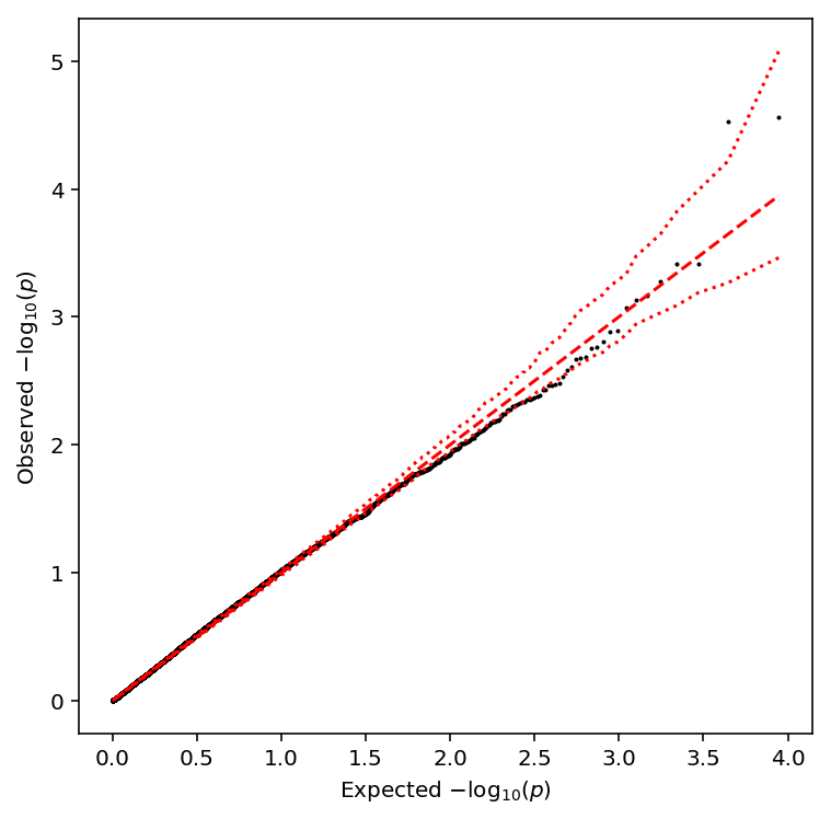
Repeat the analysis after subsetting to 54 individuals.
np.random.seed(0)
subset = np.random.choice([x for x in geuvadis.columns], size=54, replace=False)
pd.Series(subset).sort_values().to_csv('/scratch/midway2/aksarkar/singlecell/geuvadis-subset.txt', header=None, index=None)
write_pheno_file(geuvadis[subset], gene_info, '/scratch/midway2/aksarkar/singlecell/geuvadis/test.bed', prefix='')
Submitted batch job 44544326
Submitted batch job 44544018
Submitted batch job 44544375
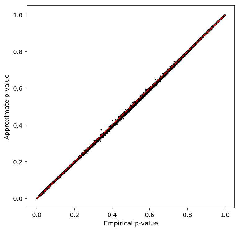
geuvadis_54_qtls = read_qtltools_output('geuvadis/test')
plot_approx_permutation(geuvadis_54_qtls)
Reproduce bulk eQTL calls
The iPSC bulk eQTLs were called in Banovich et al 2018.
eQTLs in iPSCs and LCLs: We transformed expression levels to a standard normal
within each individual. We next accounted for unknown confounders by removing
principal components from the LCL (15 PCs) and iPSC (10 PCs) data. Genotypes
were obtained using impute2 as described previously (Li et al. 2016). We only
considered variants within 50 kb of genes. To identify association between
genotype and gene expression, we used FastQTL (Ongen et al. 2016). After the
initial regression, a variable number of permutations were performed to obtain
a gene-wise adjusted P-value (Ongen et al. 2016). To identify significant
eQTLs, we used Storey's q-value (Storey and Tibshirani 2003) on the adjusted
P-values. Genes with a q-value less than 0.1 are considered significant.
Important notes:
The text doesn't state how expression level was quantified (it was the ratio of mapped reads to total reads after correction by
WASP).WASP(de Geijin et al 2015) fits quartic polynomials \(f, g\) which predict the total read count per region \(T^*_{ij}\) from the observed read count \(x_{ij}\) and GC content \(w_j\) by maximizing the likelihood of the observed read counts:\[ x_{ij} \sim \mathrm{Pois}(T^*_{ij}) \]
\[ T^*_{ij} = \exp\left(f\left(\sum_i x_{ij}\right)\right) g(w_j) \]
Using log CPM (under the assumption that we never compare genes to each other) yields 1279 eQTLs (89%).
fastqtlexpects gene start/end, and only takes cis-SNPs around the start ignoring strand. The code uses GENCODE v19 exons to define the start/end.qtltoolsexpects TSS and strand, but doesn't use strand information in cis-eQTL mapping. Using the start coordinate of the provided expression matrix as TSS yields 1265 eQTLs (87%).- The methods section of Degner et al 2012 states data is standardized across individuals, and quantile normalized within individuals. The equation contradicts the text, but the code follows the text.
- The code analyzes 100kb windows, contradicting the text.
- Not every gene in the input appears in the output, and changing the number of chunks changes the number of genes lost.
- QTL-gene pairs passed the Benjamini-Hochberg procedure, not Storey's procedure.
sbatch --partition=broadwl -a 1-25
#!/bin/bash
source activate scqtl
fastqtl -V YRI_SNPs_2_IPSC.txt.gen.gz -B fastqtl_qqnorm_RNAseq_run.fixed.txt.gz -C fasteqtl_PC_RNAseq_run.fixed.txt -O bulk-qtl.$SLURM_ARRAY_TASK_ID.txt --exclude-samples file_IPSC.excl --window 1e5 --permute 1000 10000 --chunk $SLURM_ARRAY_TASK_ID 25 --seed 1475098497
Submitted batch job 44546060
Subsample the individuals.
sbatch --partition=broadwl -a 1-25
#!/bin/bash
source activate scqtl
awk 'NR < 6' file_IPSC.used | cat - file_IPSC.excl >subsample.excl
fastqtl -V YRI_SNPs_2_IPSC.txt.gen.gz -B fastqtl_qqnorm_RNAseq_run.fixed.txt.gz -C fasteqtl_PC_RNAseq_run.fixed.txt -O bulk-qtl.$SLURM_ARRAY_TASK_ID.txt --exclude-samples subsample.excl --window 1e5 --permute 1000 10000 --chunk $SLURM_ARRAY_TASK_ID 25 --seed 1475098497
Submitted batch job 47297158
Read fastqtl output.
bulk_qtls = read_fastqtl_output('reproduce-yang/bulk')
Write out the summary stats with headers.
bulk_qtls.to_csv('/project2/mstephens/aksarkar/projects/singlecell-qtl/data/scqtl-mapping/bulk.txt.gz', sep='\t', index=None, compression='gzip')
Compare qtltools to fastqtl. The input files need to be modified.
sbatch --partition=broadwl --wait
#!/bin/bash
zcat fastqtl_qqnorm_RNAseq_run.fixed.txt.gz | awk -vOFS='\t' 'NR == 1 {$4 = "pid" OFS "gid" OFS "strand"; for (i = 5; i <= NF; i++) {$i = "NA"$i} print} NR > 1 {$4 = $4 OFS $4 OFS "+"; $3 = $2; print}' >test.bed
awk 'NR == 1 {for (i = 2; i <= NF; i++) {$i = "NA"$i}} {print}' fasteqtl_PC_RNAseq_run.fixed.txt >bulk-covars.txt
Submitted batch job 44979838
Check whether the FDR is properly controlled by permuting.
np.random.seed(0)
permutation = bulk_expr.columns.values.copy()
np.random.shuffle(permutation[5:])
bulk_expr.columns = permutation

covars = (pd.read_table('/scratch/midway2/aksarkar/singlecell/reproduce-yang/covars.txt', sep=' ')
          .rename(columns={k: v for k, v in zip(bulk_expr.columns, permutation)}))
covars.to_csv('/scratch/midway2/aksarkar/singlecell/reproduce-yang/covars.txt', sep=' ', index=False)
Fix the TSS by rewriting the phenotype file.
bulk_expr = pd.read_table('/scratch/midway2/aksarkar/singlecell/reproduce-yang/test.bed', index_col=3)
bulk_expr.index = [x.split('.')[0] for x in bulk_expr.index]
write_pheno_file(bulk_expr.iloc[:,5:], gene_info, '/scratch/midway2/aksarkar/singlecell/reproduce-yang/test.bed', holdout=False)
Index the phenotype file.
Submitted batch job 44683584
Run qtltools.
Submitted batch job 44683586
Run qtltools on reprocessed dosages.
Submitted batch job 47427752
Run qtltools on subsample.
awk '{print "NA" $0}' subsample.excl >subsample-qtltools.excl
Submitted batch job 47428279
Read qtltools output
bulk_qtls = read_qtltools_output('reproduce-yang/test')
Check the beta approximation.
plot_approx_permutation(bulk_qtls)
Plot a QQ plot of adjusted p-values.
qqplot(bulk_qtls)
Take QTLs with \(\mathrm{FDR} < 0.1\).
bulk_qtls['fdr_pass'].sum()
1136
Recall bulk eQTLs from log CPM
Read the counts matrix.
bulk_counts = (pd.read_table('/project2/gilad/singlecell-qtl/bulk/counts_RNAseq_iPSC.txt', sep=' ', index_col=0)
               .rename(columns=lambda x: 'NA{}'.format(x))
               .rename(index=lambda x: x.split('.')[0]))
Throw out individuals.
with open('/scratch/midway2/aksarkar/singlecell/reproduce-yang/file_IPSC.excl') as f:
  for line in f:
    k = 'NA{}'.format(line.strip())
    if k in bulk_counts:
      del bulk_counts[k]
Normalize the counts matrix by computing log CPM. Normalizing by length is unnecessary because we only ever compare counts for the same gene across individuals.
bulk_log_cpm = (cpm(bulk_counts)
                .transform(lambda x: (x - x.mean()) / x.std(), axis=1)
                .apply(qqnorm, axis=0))
Compute expression PCs.
covars = pd.DataFrame(skd.PCA(n_components=10).fit(bulk_log_cpm).components_, columns=bulk_log_cpm.columns)
covars.index.name = 'id'
covars.to_csv('/scratch/midway2/aksarkar/singlecell/recall-bulk/log-cpm-covars.txt', sep='\t')
Check whether the false discovery rate is properly controlled by permuting the data.
Write the phenotype matrix in qtltools format. Use the annotation data
(ENSEMBL 75) in this repository to be consistent with the single cell
data. Important: this loses 1716 genes (are they pseudogenes?)
write_pheno_file(
  bulk_log_cpm,
  gene_info,
  holdout=False,
  output_file='/scratch/midway2/aksarkar/singlecell/recall-bulk/bulk-log-cpm.bed')
Index the phenotype file.
Submitted batch job 44681764
Ensure the dosage file follows the VCF standard. Add the prefix NA to sample IDs.
sbatch --partition=broadwl
#!/bin/bash
zcat YRI_SNPs_2_IPSC.txt.gen.gz | awk -vOFS='\t' 'BEGIN {print "##fileformat=VCFv4.2"; print "##FORMAT=<ID=DS,Number=1,Type=Float>"} NR == 1 {for (i = 10; i <= NF; i++) {$i = "NA"$i}} {print}' | bgzip >yri-dosages.vcf.gz
tabix yri-dosages.vcf.gz
Submitted batch job 44546926
Run qtltools
Submitted batch job 44681768
Read the output. Important: this loses 201 genes (is this a bug in
qtltools)?
bulk_cpm_qtls = read_qtltools_output('recall-bulk/bulk-log-cpm')
Check the beta approximation.
plot_approx_permutation(bulk_cpm_qtls)
Plot a QQ plot of adjusted p-values.
qqplot(bulk_cpm_qtls)
Take QTLs with \(\mathrm{FDR} < 0.1\).
bulk_cpm_qtls['fdr_pass'].sum()
1276
Recall bulk eQTLs from log TPM
We reprocessed the bulk RNA-Seq data using kallisto. Read the TPM
matrix.
bulk_log_tpm = pd.read_table('/project2/mstephens/aksarkar/projects/singlecell-qtl/data/kallisto/bulk-ipsc-tpm.txt.gz', header=None, sep=' ')
bulk_log_tpm = np.log(bulk_log_tpm.pivot(columns=0, index=1, values=2) + 1)
bulk_log_tpm.index = [x.split('.')[0] for x in bulk_log_tpm.index]
# Important: need to throw out all zero rows because they blow up
# standardization
bulk_log_tpm = (bulk_log_tpm[bulk_log_tpm.apply(lambda x: x.sum() > 0, axis=1)]
                .transform(lambda x: (x - x.mean()) / x.std(), axis=1)
                .apply(qqnorm, axis=0))
To quantify how much power we expect to lose going from 58 to 53 individuals (in our scRNA-Seq data), perform QTL mapping on a random subset of 53 individuals.
np.random.seed(0)
keep_inds = np.random.choice(bulk_log_tpm.columns, size=53, replace=False)
bulk_log_tpm = bulk_log_tpm.filter(items=keep_inds, axis='columns')
Get the TSS information. Use the annotation data (ENSEMBL 75) in this repository to be consistent with the single cell data.
Write the phenotype matrix in qtltools format. Important: this loses 1034
genes
write_pheno_file(
  bulk_log_tpm,
  gene_info,
  holdout=False,
  output_file='/scratch/midway2/aksarkar/singlecell/recall-bulk/bulk-log-tpm.bed')
Index the phenotype file.
Submitted batch job 47427500
Compute principal components.
covars = pd.DataFrame(skd.PCA(n_components=6).fit(bulk_log_tpm).components_, columns=bulk_log_tpm.columns)
covars.index.name = 'id'
covars.to_csv('/scratch/midway2/aksarkar/singlecell/recall-bulk/log-tpm-covars.txt', sep='\t')
Run qtltools
Submitted batch job 47427616
Read the output. Important: this loses 201 genes (is this a bug in
qtltools)?
bulk_tpm_qtls = read_qtltools_output('recall-bulk/bulk-log-tpm')
Check the beta approximation to the permuted p-values.
plot_approx_permutation(bulk_tpm_qtls)
Plot a QQ plot of the adjusted p-values.
qqplot(bulk_tpm_qtls)
Take QTLs with \(\mathrm{FDR} < 0.1\).
bulk_tpm_qtls['fdr_pass'].sum()
683
Reprocess YRI dosages
We have two individuals which weren't used in Banovich et al 2018, so we don't have their genotypes. Reprocess the IMPUTE2 output to get the correct dosage matrix.
rsync -au -f '+ */' -f '+ *.impute2.gz' -f '+ YRI_samples.txt' -f '- *' /mnt/lustre/data/internal/genotypes/hg19/YRI/ aksarkar@midway2.rcc.uchicago.edu:/scratch/midway2/aksarkar/singlecell/scqtl-mapping/
import argparse
import glob
import gzip
import numpy as np
import pandas as pd
import sqlite3

def convert_impute2_vcf(file, chrom, outfile, min_maf=0.05, mask=None):
  for line in file:
    record = line.split()
    posterior = np.array([float(x) for x in record[5:]])
    dose = posterior.reshape(-1, 3).dot(np.arange(3))
    if mask is not None:
      dose = dose[mask]
    if min_maf <= dose.mean() / 2 <= 1 - min_maf:
      print(chrom, record[2], '{}.{}.{}'.format(record[1], chrom, record[2]),
            record[3], record[4], '.', '.', '.', 'DS',
            *['{:.3f}'.format(x) for x in dose], sep='\t', file=outfile)

parser = argparse.ArgumentParser()
parser.add_argument('-s', '--subset', help='Sample inclusion list', type=pd.read_table, default=None)
parser.add_argument('-o', '--output', help='Output file', default='dosages.vcf')
args = parser.parse_args()

samples = pd.read_table('YRI_samples.txt', header=None, sep=' ')
if args.subset is not None:
  mask = samples[0].isin(args.subset).values
  samples = samples.loc[mask.values.ravel(), 0]
else:
  mask = None
  samples = samples.loc[:,0]
with open(args.output, 'w') as f:
  print('##fileformat=VCFv4.2', file=f)
  print('##FORMAT=<ID=DS,Number=1,Type=Float>', file=f)
  print('#CHROM', 'POS', 'ID', 'REF', 'ALT', 'QUAL', 'FILTER', 'INFO', 'FORMAT', *samples, sep='\t', file=f)
  for c in range(1, 23):
    with gzip.open('chr{}.hg19.impute2.gz'.format(c), 'rt') as g:
      convert_impute2_vcf(g, 'chr{}'.format(c), outfile=f, mask=mask)
sbatch --partition=broadwl -n1 -c28 --exclusive --mem=8G
#!/bin/bash
source activate scqtl
python /project2/mstephens/aksarkar/projects/singlecell-qtl/code/reprocess-dosage.py -o yri-120-dosages.vcf
bgzip --threads=28 yri-120-dosages.vcf
tabix yri-120-dosages.vcf.gz
Submitted batch job 47228636
Analysis using counts
One obvious way to estimate means/variances to use as quantitative phenotypes is to use the sample means/variances of the counts.
Call eQTLs from pooled scRNA-Seq
Read the QC filters.
annotation = pd.read_table('/project2/mstephens/aksarkar/projects/singlecell-qtl/data/scqtl-annotation.txt')
keep_samples = pd.read_table('/project2/mstephens/aksarkar/projects/singlecell-qtl/data/quality-single-cells.txt', index_col=0, header=None)
keep_genes = pd.read_table('/project2/mstephens/aksarkar/projects/singlecell-qtl/data/genes-pass-filter.txt', index_col=0, header=None)
annotation = annotation.loc[keep_samples.values.ravel()]
keep_inds = annotation.groupby('chip_id').apply(lambda x: len(x) >= 50)
Read and pool the UMI data.
pooled_counts = pd.concat(
  [(chunk
    .filter(items=keep_genes[keep_genes.values].index, axis='index')
    # Important: this can't be done by filter because sample names are
    # different in the QC file
    .loc[:,keep_samples.values.ravel()]
    .groupby(annotation['chip_id'].values, axis=1)
    .agg(np.sum))
   for chunk in
   pd.read_table('/project2/mstephens/aksarkar/projects/singlecell-qtl/data/scqtl-counts.txt.gz',
                 chunksize=1000, index_col=0)])
Normalize the pooled counts.
pooled_counts = (pooled_counts.loc[:,keep_inds]
              .transform(lambda x: (x - x.mean()) / x.std(), axis=1)
              .apply(qqnorm, axis=0))
Compute principal components and write out the covariate file.
covars = pd.DataFrame(skd.PCA(n_components=10).fit(pooled_counts).components_, columns=pooled_counts.columns)
covars.index.name = 'id'
covars.to_csv('/scratch/midway2/aksarkar/singlecell/scqtl-mapping/counts/pooled-covars.txt', sep='\t')
Write out the phenotype file.
write_pheno_file(pooled_counts, gene_info, holdout=False, output_file='/scratch/midway2/aksarkar/singlecell/scqtl-mapping/counts/pooled.bed')
Index the phenotype file.
Submitted batch job 55769711
Run qtltools
Read the output. Important: this loses 200 genes (is this a bug in
qtltools)?
pooled_qtls = read_qtltools_output('scqtl-mapping/counts/pooled')
Check the beta approximation.
plot_approx_permutation(pooled_qtls)
Plot a QQ plot of the adjusted p-values.
qqplot(pooled_qtls)
Take QTLs with \(\mathrm{FDR} < 0.1\).
pooled_qtls['fdr_pass'].sum()
231
Call mean-QTLs
Read the count matrix.
umi = pd.concat(
  [(chunk
    .filter(items=keep_genes[keep_genes.values].index, axis='index')
    # Important: this can't be done by filter because sample names are
    # different in the QC file
    .loc[:,keep_samples.values.ravel()])
   for chunk in
   pd.read_table('/project2/mstephens/aksarkar/projects/singlecell-qtl/data/scqtl-counts.txt.gz',
                 chunksize=1000, index_col=0)])
Compute the sample mean per individual, then normalize.
sample_mean = (umi
               .groupby(annotation['chip_id'].values, axis=1)
               .agg(np.mean)
               .transform(lambda x: (x - x.mean()) / x.std(), axis=1)
               .apply(qqnorm, axis=0))
Compute principal components and write out the covariate file.
covars = pd.DataFrame(skd.PCA(n_components=10).fit(sample_mean).components_, columns=sample_mean.columns)
covars.index.name = 'id'
covars.to_csv('/scratch/midway2/aksarkar/singlecell/scqtl-mapping/counts/sample-mean-covars.txt', sep='\t')
Write out the phenotype file for qtltools. Hold out even chromosomes while
optimizing the power to detect eQTLs.
write_pheno_file(
  sample_mean,
  gene_info,
  output_file='/scratch/midway2/aksarkar/singlecell/scqtl-mapping/counts/sample-mean.bed',
  holdout=False)
Index the phenotype file.
Submitted batch job 55770738
Run qtltools.
Submitted batch job 55770741
Read the output.
sample_mean_qtls = read_qtltools_output('scqtl-mapping/counts/sample-mean')
Check the beta approximation to the permutation p-values.
plot_approx_permutation(sample_mean_qtls)
Plot a QQ plot of the adjusted p-values.
qqplot(sample_mean_qtls)
Take QTLs at FDR 10%.
sample_mean_qtls['fdr_pass'].sum()
268
Call variance-QTLs
Read the UMI matrix.
Compute the sample variance per individual, then normalize.
sample_var = (umi
              .groupby(annotation['chip_id'].values, axis=1)
              .agg(np.var)
              .transform(lambda x: (x - x.mean()) / x.std(), axis=1)
              .apply(qqnorm, axis=0))
Compute principal components and write out the covariate file.
covars = pd.DataFrame(skd.PCA(n_components=2).fit(sample_var).components_, columns=sample_var.columns)
covars.index.name = 'id'
covars.to_csv('/scratch/midway2/aksarkar/singlecell/scqtl-mapping/counts/sample-var-covars.txt', sep='\t')
Write out the phenotype file for qtltools. Hold out even chromosomes while
optimizing the power to detect eQTLs.
write_pheno_file(sample_var, gene_info, '/scratch/midway2/aksarkar/singlecell/scqtl-mapping/counts/sample-var.bed', holdout=False)
Index the phenotype file.
Submitted batch job 55770997
Run qtltools.
Submitted batch job 55771003
Read the output.
sample_var_qtls = read_qtltools_output('scqtl-mapping/counts/sample-var')
Check the beta approximation to the permutation p-values.
plot_approx_permutation(sample_var_qtls)
Plot a QQ plot of the adjusted p-values.
qqplot(sample_var_qtls)
Take QTLs at FDR 10%.
sample_var_qtls['fdr_pass'].sum()
94
Call CV-QTLs
Compute the sample CV per individual per gene, then normalize.
sample_cv = (umi
             .groupby(annotation['chip_id'].values, axis=1)
             .agg(lambda x: np.std(x, axis=1) / (np.mean(x, axis=1) + 1e-8))
             .transform(lambda x: (x - x.mean()) / x.std(), axis=1)
             .apply(qqnorm, axis=0))
Write out the phenotype file for qtltools. Hold out even chromosomes while
optimizing the power to detect eQTLs.
write_pheno_file(sample_cv, gene_info, '/scratch/midway2/aksarkar/singlecell/scqtl-mapping/counts/sample-cv.bed', holdout=False)
Index the phenotype file.
Submitted batch job 55771641
Run qtltools.
Submitted batch job 55771671
Read the output.
sample_cv_qtls = read_qtltools_output('scqtl-mapping/counts/sample-cv')
Check the beta approximation to the permutation p-values.
plot_approx_permutation(sample_cv_qtls)
Plot a QQ plot of the adjusted p-values.
qqplot(sample_cv_qtls)
Take QTLs at FDR 10%.
sample_cv_qtls['fdr_pass'].sum()
4
Call Fano-QTLs
Read the UMI matrix.
Compute the sample Fano factor per individual per gene, then normalize.
sample_fano = (umi
               .groupby(annotation['chip_id'].values, axis=1)
               .agg(lambda x: np.var(x, axis=1) / (1e-8 + np.mean(x, axis=1)))
               .transform(lambda x: (x - x.mean()) / x.std(), axis=1)
               .apply(qqnorm, axis=0))
Write out the phenotype file for qtltools. Hold out even chromosomes while
optimizing the power to detect eQTLs.
write_pheno_file(sample_fano, gene_info, '/scratch/midway2/aksarkar/singlecell/scqtl-mapping/counts/sample_fano.bed', holdout=False)
Index the phenotype file.
Submitted batch job 55771840
Compute principal components and write out the covariate file.
covars = pd.DataFrame(skd.PCA(n_components=2).fit(sample_fano).components_, columns=sample_fano.columns)
covars.index.name = 'id'
covars.to_csv('/scratch/midway2/aksarkar/singlecell/scqtl-mapping/counts/sample-fano-covars.txt', sep='\t')
Run qtltools.
Submitted batch job 55771844
Read the output.
sample_fano_qtls = read_qtltools_output('scqtl-mapping/counts/sample_fano')
Check the beta approximation to the permutation p-values.
plot_approx_permutation(sample_fano_qtls)

Plot a QQ plot of the adjusted p-values.
qqplot(sample_fano_qtls)
Take QTLs at FDR 10%.
sample_fano_qtls['fdr_pass'].sum()
11
Analysis using log CPM
The most obvious way to estimate means/variances to use as quantitative phenotypes is to use the sample moments of per cell log CPM.
Care has to be taken in handling zero-observations. Simply ignoring them leads to loss of power due to the pseudocount introduced in computing log CPM. To see this, fix one individual, one gene, and let \(r\) denote the observed count. Then,
\[ \log\mathrm{CPM} \propto \ln(r + \epsilon) - \ln\mathrm{const} \]
Let \(\mu = \mathbb{E}[r\,]\), \(\sigma^2 = \mathbb{V}[r\,]\), expand to second-order, then take expectations over cells:
\[ \mathbb{E}[\,\ln (r + \epsilon)\,] \approx \ln(\mu + \epsilon) - \frac{\sigma^2}{(\mu + \epsilon)^2} \]
\[ \mathbb{V}[\,\ln (r + \epsilon)\,] \approx \frac{2 \sigma^2}{(\mu + \epsilon)^2} - \frac{\sigma^4}{(\mu + \epsilon)^4} \]
Call eQTLs from pooled scRNA-Seq
Read the QC filters.
annotation = pd.read_table('/project2/mstephens/aksarkar/projects/singlecell-qtl/data/scqtl-annotation.txt')
keep_samples = pd.read_table('/project2/mstephens/aksarkar/projects/singlecell-qtl/data/quality-single-cells.txt', index_col=0, header=None)
keep_genes = pd.read_table('/project2/mstephens/aksarkar/projects/singlecell-qtl/data/genes-pass-filter.txt', index_col=0, header=None)
annotation = annotation.loc[keep_samples.values.ravel()]
keep_inds = annotation.groupby('chip_id').apply(lambda x: len(x) >= 50)
Read and pool the UMI data.
pooled_counts = pd.concat(
  [(chunk
    .filter(items=keep_genes[keep_genes.values].index, axis='index')
    # Important: this can't be done by filter because sample names are
    # different in the QC file
    .loc[:,keep_samples.values.ravel()]
    .groupby(annotation['chip_id'].values, axis=1)
    .agg(np.sum))
   for chunk in
   pd.read_table('/project2/mstephens/aksarkar/projects/singlecell-qtl/data/scqtl-counts.txt.gz',
                 chunksize=1000, index_col=0)])
Normalize the pooled counts.
pooled_cpm = (cpm(pooled_counts).loc[:,keep_inds]
              .transform(lambda x: (x - x.mean()) / x.std(), axis=1)
              .apply(qqnorm, axis=0))
Compute principal components and write out the covariate file.
covars = pd.DataFrame(skd.PCA(n_components=10).fit(pooled_cpm).components_, columns=pooled_cpm.columns)
covars.index.name = 'id'
covars.to_csv('/scratch/midway2/aksarkar/singlecell/scqtl-mapping/counts/pooled-covars.txt', sep='\t')
Write out the phenotype file.
write_pheno_file(pooled_cpm, gene_info, holdout=False, output_file='/scratch/midway2/aksarkar/singlecell/scqtl-mapping/counts/pooled.bed')
Index the phenotype file.
Submitted batch job 55767633
Run qtltools
Read the output. Important: this loses 200 genes (is this a bug in
qtltools)?
pooled_qtls = read_qtltools_output('scqtl-mapping/counts/pooled')
Check the beta approximation.
plot_approx_permutation(pooled_qtls)
Plot a QQ plot of the adjusted p-values.
qqplot(pooled_qtls)
Take QTLs with \(\mathrm{FDR} < 0.1\).
pooled_qtls['fdr_pass'].sum()
261
Call mean-QTLs
Throw out individuals with fewer than 50 cells.
Read the count matrix.
umi = pd.concat(
  [(chunk
    .filter(items=keep_genes[keep_genes.values].index, axis='index')
    # Important: this can't be done by filter because sample names are
    # different in the QC file
    .loc[:,keep_samples.values.ravel()])
   for chunk in
   pd.read_table('/project2/mstephens/aksarkar/projects/singlecell-qtl/data/scqtl-counts.txt.gz',
                 chunksize=1000, index_col=0)])
We previously noted that 50 cells was sufficient to reliably estimate the mean of single cell data. Therefore, throw out zeros from the analysis and require that at least 50 samples have non-zero count.
num_non_zero = umi.groupby(annotation['chip_id'].values, axis=1).agg(lambda x: (x > 0).values.sum(axis=1))
Derive a cutoff for the number of individuals with at least 50 non-zero observations per gene.
num_individuals_pass = (num_non_zero > 50).agg(np.sum, axis=1)
plt.clf()
n, b, _ = plt.hist(num_individuals_pass, color='k', bins=np.arange(0, 53, 2), histtype='step', cumulative=True, normed=True)
plt.axhline(y=n[-2], c='r', ls=':', lw=1)
plt.xlabel('Number of individuals with at least 50 non-zero observations')
_ = plt.ylabel('Cumulative fraction of genes')

Compute the sample mean log CPM per individual, then normalize.
sample_mean = (cpm(umi)
               .mask(umi == 0)
               .groupby(annotation['chip_id'].values, axis=1)
               .agg(np.mean)
               .loc[num_individuals_pass >= 50,keep_inds]
               .transform(lambda x: (x - x.mean()) / x.std(), axis=1)
               .apply(qqnorm, axis=0))
Compute principal components and write out the covariate file.
covars = pd.DataFrame(skd.PCA(n_components=10).fit(sample_mean).components_, columns=sample_mean.columns)
covars.index.name = 'id'
covars.to_csv('/scratch/midway2/aksarkar/singlecell/scqtl-mapping/counts/sample-mean-covars.txt', sep='\t')
Write out the phenotype file for qtltools. Hold out even chromosomes while
optimizing the power to detect eQTLs.
write_pheno_file(
  sample_mean,
  gene_info,
  output_file='/scratch/midway2/aksarkar/singlecell/scqtl-mapping/counts/sample-mean.bed',
  holdout=False)
Index the phenotype file.
Submitted batch job 55768305
Run qtltools.
Submitted batch job 46254485
Read the output.
sample_mean_qtls = read_qtltools_output('scqtl-mapping/counts/sample-mean')
Check the beta approximation to the permutation p-values.
plot_approx_permutation(sample_mean_qtls)
Plot a QQ plot of the adjusted p-values.
qqplot(sample_mean_qtls)
Take QTLs at FDR 10%.
sample_mean_qtls['fdr_pass'].sum()
207
Call variance-QTLs
Throw out individuals with fewer than 50 cells.
Read the UMI matrix.
Compute the sample variance of log CPM per individual, then normalize.
sample_var = (cpm(umi)
              .mask(umi == 0)
              .groupby(annotation['chip_id'].values, axis=1)
              .agg(np.var)
              .loc[num_individuals_pass >= 50,keep_inds]
              .transform(lambda x: (x - x.mean()) / x.std(), axis=1)
              .apply(qqnorm, axis=0))
Compute principal components and write out the covariate file.
covars = pd.DataFrame(skd.PCA(n_components=2).fit(sample_var).components_, columns=sample_var.columns)
covars.index.name = 'id'
covars.to_csv('/scratch/midway2/aksarkar/singlecell/scqtl-mapping/counts/sample-var-covars.txt', sep='\t')
Write out the phenotype file for qtltools. Hold out even chromosomes while
optimizing the power to detect eQTLs.
write_pheno_file(sample_var, gene_info, '/scratch/midway2/aksarkar/singlecell/scqtl-mapping/counts/sample-var.bed', holdout=False)
Index the phenotype file.
Submitted batch job 55769014
Run qtltools.
Submitted batch job 55769016
Read the output.
sample_var_qtls = read_qtltools_output('scqtl-mapping/counts/sample-var')
Check the beta approximation to the permutation p-values.
plot_approx_permutation(sample_var_qtls)
Plot a QQ plot of the adjusted p-values.
qqplot(sample_var_qtls)
Take QTLs at FDR 10%.
sample_var_qtls['fdr_pass'].sum()
0
Call CV-QTLs
Throw out individuals with fewer than 50 cells.
Read the UMI matrix.
Compute the sample CV of log CPM per individual, then normalize.
sample_cv = (cpm(umi)
             .mask(umi == 0)
             .groupby(annotation['chip_id'].values, axis=1)
             .agg(lambda x: np.std(x, axis=1) / (np.mean(x, axis=1) + 1e-8))
             .loc[num_individuals_pass >= 50,keep_inds]
             .transform(lambda x: (x - x.mean()) / x.std(), axis=1)
             .apply(qqnorm, axis=0))
Write out the phenotype file for qtltools. Hold out even chromosomes while
optimizing the power to detect eQTLs.
write_pheno_file(sample_cv, gene_info, '/scratch/midway2/aksarkar/singlecell/scqtl-mapping/counts/sample-cv.bed', holdout=False)
Index the phenotype file.
Submitted batch job 55769280
Run qtltools.
Submitted batch job 55769282
Read the output.
sample_cv_qtls = read_qtltools_output('scqtl-mapping/counts/sample-cv')
Check the beta approximation to the permutation p-values.
plot_approx_permutation(sample_cv_qtls)
Plot a QQ plot of the adjusted p-values.
qqplot(sample_cv_qtls)
Take QTLs at FDR 10%.
sample_cv_qtls['fdr_pass'].sum()
3
Call Fano-QTLs
Throw out individuals with fewer than 50 cells.
Read the UMI matrix.
Fisher's index of dispersion is defined as \(V[x] / E[x]\). The Fano factor is Fisher's index of dispersion over a fixed window (in our case, the total number of reads).
Compute the sample Fano factor of log CPM per individual, then normalize.
sample_fano = (cpm(umi)
               .mask(umi == 0)
               .groupby(annotation['chip_id'].values, axis=1)
               .agg(lambda x: np.var(x, axis=1) / (np.mean(x, axis=1)))
               .loc[num_individuals_pass >= 50,keep_inds]
               .transform(lambda x: (x - x.mean()) / x.std(), axis=1)
               .apply(qqnorm, axis=0))
Write out the phenotype file for qtltools. Hold out even chromosomes while
optimizing the power to detect eQTLs.
write_pheno_file(sample_fano, gene_info, '/scratch/midway2/aksarkar/singlecell/scqtl-mapping/counts/sample_fano.bed', holdout=False)
Index the phenotype file.
Submitted batch job 55769523
Compute principal components and write out the covariate file.
covars = pd.DataFrame(skd.PCA(n_components=2).fit(sample_fano).components_, columns=sample_fano.columns)
covars.index.name = 'id'
covars.to_csv('/scratch/midway2/aksarkar/singlecell/scqtl-mapping/counts/sample-fano-covars.txt', sep='\t')
Run qtltools.
Submitted batch job 55769526
Read the output.
sample_fano_qtls = read_qtltools_output('scqtl-mapping/counts/sample_fano')
Check the beta approximation to the permutation p-values.
plot_approx_permutation(sample_fano_qtls)
Plot a QQ plot of the adjusted p-values.
qqplot(sample_fano_qtls)
Take QTLs at FDR 10%.
sample_fano_qtls['fdr_pass'].sum()
0
Analysis using ZINB
Call eQTLs
Estimate the moments of latent gene expression. We have:
\[ \mathbb{E}[\lambda_{ijk}] = (1 - \pi_{ik}) \mu_{ik} \]
\[ \mathbb{V}[\lambda_{ijk}] = (1 - \pi_{ik}) \phi_{ik}^{-1} + \pi_{ik} (1 - \pi_{ik}) \mu_{ik}^2 \]
log_mu = pd.read_table('/project2/mstephens/aksarkar/projects/singlecell-qtl/data/density-estimation/design1/zi2-log-mu.txt.gz', index_col=0, sep=' ')
log_phi = pd.read_table('/project2/mstephens/aksarkar/projects/singlecell-qtl/data/density-estimation/design1/zi2-log-phi.txt.gz', index_col=0, sep=' ')
logodds = pd.read_table('/project2/mstephens/aksarkar/projects/singlecell-qtl/data/density-estimation/design1/zi2-logodds.txt.gz', index_col=0, sep=' ')
for x in (log_mu, log_phi, logodds):
  del x['NA18498']

# Important: log(sigmoid(x)) = -softplus(-x)
mean_by_ind = np.exp(log_mu - np.log1p(np.exp(logodds)))
variance_by_ind = np.exp(2 * log_mu + log_phi - np.log1p(np.exp(logodds))) + np.exp(-np.log1p(np.exp(logodds)) - np.log1p(np.exp(-logodds)) + 2 * log_mu)
Normalize the mean matrix analagous to the bulk data.
mean = (mean_by_ind
        .transform(lambda x: (x - x.mean()) / x.std(), axis=1)
        .apply(qqnorm, axis=0))
Compute principal components of the mean matrix.
covars = pd.DataFrame(skd.PCA(n_components=10).fit(mean).components_, columns=mean.columns)
covars.index.name = 'id'
covars.to_csv('/scratch/midway2/aksarkar/singlecell/scqtl-mapping/zinb/mean-covars.txt', sep='\t')
Write out the phenotype file for qtltools. Hold out even chromosomes while
optimizing the power to detect eQTLs.
write_pheno_file(mean, gene_info, '/scratch/midway2/aksarkar/singlecell/scqtl-mapping/zinb/mean.bed', holdout=False)
Index the phenotype file.
Submitted batch job 55772051
Run qtltools.
Submitted batch job 55772076
Read the output.
mean_qtls = read_qtltools_output('scqtl-mapping/zinb/mean')
Check the beta approximation to the permutation p-values.
plot_approx_permutation(mean_qtls)

Plot a QQ plot of the adjusted p-values.
qqplot(mean_qtls)

Take QTLs at FDR 10%.
mean_qtls['fdr_pass'].sum()
235
Fit multiplicative model
Estimate the moments of latent gene expression. We have:
\[ \mathbb{E}[\lambda_{ijk}] = (1 - \pi_{ik}) \mu_{ik} \]
\[ \mathbb{V}[\lambda_{ijk}] = (1 - \pi_{ik}) \phi_{ik}^{-1} + \pi_{ik} (1 - \pi_{ik}) \mu_{ik}^2 \]
log_mu = pd.read_table('/project2/mstephens/aksarkar/projects/singlecell-qtl/data/density-estimation/design1/zi2-log-mu.txt.gz', index_col=0, sep=' ')
log_phi = pd.read_table('/project2/mstephens/aksarkar/projects/singlecell-qtl/data/density-estimation/design1/zi2-log-phi.txt.gz', index_col=0, sep=' ')
logodds = pd.read_table('/project2/mstephens/aksarkar/projects/singlecell-qtl/data/density-estimation/design1/zi2-logodds.txt.gz', index_col=0, sep=' ')
for x in (log_mu, log_phi, logodds):
  del x['NA18498']

# Important: log(sigmoid(x)) = -softplus(-x)
mean_by_ind = np.exp(log_mu - np.log1p(np.exp(logodds)))
variance_by_ind = np.exp(2 * log_mu + log_phi - np.log1p(np.exp(logodds))) + np.exp(-np.log1p(np.exp(logodds)) - np.log1p(np.exp(-logodds)) + 2 * log_mu)
Normalize the mean matrix analagous to the bulk data.
multmean = (np.log(mean_by_ind)
        .transform(lambda x: (x - x.mean()) / x.std(), axis=1)
        .apply(qqnorm, axis=0))
Compute principal components of the mean matrix.
covars = pd.DataFrame(skd.PCA(n_components=10).fit(multmean).components_, columns=multmean.columns)
covars.index.name = 'id'
covars.to_csv('/scratch/midway2/aksarkar/singlecell/scqtl-mapping/zinb/multmean-covars.txt', sep='\t')
Write out the phenotype file for qtltools. Hold out even chromosomes while
optimizing the power to detect eQTLs.
write_pheno_file(multmean, gene_info, '/scratch/midway2/aksarkar/singlecell/scqtl-mapping/zinb/multmean.bed', holdout=False)
Index the phenotype file.
Submitted batch job 55772263
Run qtltools.
Submitted batch job 55772298
Read the output.
multmean_qtls = read_qtltools_output('scqtl-mapping/zinb/mean')
Check the beta approximation to the permutation p-values.
plot_approx_permutation(multmean_qtls)
Plot a QQ plot of the adjusted p-values.
qqplot(multmean_qtls)

Take QTLs at FDR 10%.
multmean_qtls['fdr_pass'].sum()
235
Call φ-QTLs
Normalize the phenotype matrix.
log_phi = log_phi.transform(lambda x: (x - x.mean()) / x.std(), axis=1).apply(qqnorm, axis=1)
Write out the phenotype file.
write_pheno_file(log_phi, gene_info, holdout=False, output_file='/scratch/midway2/aksarkar/singlecell/scqtl-mapping/zinb/log_phi.bed')
Index the phenotype file.
Submitted batch job 55772635
Run qtltools.
Submitted batch job 55772639
Read the output.
log_phi_qtls = read_qtltools_output('scqtl-mapping/zinb/log_phi')
Check the beta approximation to the permutation p-values.
plot_approx_permutation(log_phi_qtls)
Plot a QQ plot of the adjusted p-values.
qqplot(log_phi_qtls)
Take QTLs at FDR 10%.
log_phi_qtls['fdr_pass'].sum()
0
Call variance-QTLs
Normalize the variance matrix.
variance = (variance_by_ind
            .transform(lambda x: (x - x.mean()) / x.std(), axis=1)
            .apply(qqnorm, axis=0))
Compute principal components of the variance matrix.
covars = pd.DataFrame(skd.PCA(n_components=2).fit(variance).components_, columns=variance.columns)
covars.index.name = 'id'
covars.to_csv('/scratch/midway2/aksarkar/singlecell/scqtl-mapping/zinb/variance-covars.txt', sep='\t')
Write out the phenotype file for qtltools.
write_pheno_file(variance, gene_info, '/scratch/midway2/aksarkar/singlecell/scqtl-mapping/zinb/variance.bed', holdout=False)
Index the phenotype file.
Submitted batch job 55772747
Run qtltools.
Submitted batch job 55772752
Read the output.
variance_qtls = read_qtltools_output('scqtl-mapping/zinb/variance')
Check the beta approximation to the permutation p-values.
plot_approx_permutation(variance_qtls)
Plot a QQ plot of the adjusted p-values.
qqplot(variance_qtls)
Take QTLs at FDR 10%.
variance_qtls['fdr_pass'].sum()
5
Call CV-QTLs
Estimate the coefficient of variation.
cv = np.sqrt(variance_by_ind) / mean_by_ind
Normalize the CV matrix.
cv = cv.transform(lambda x: (x - x.mean()) / x.std(), axis=1).apply(qqnorm, axis=0)
Write out the phenotype file for qtltools. Hold out even chromosomes while
optimizing the power to detect eQTLs.
write_pheno_file(cv, gene_info, '/scratch/midway2/aksarkar/singlecell/scqtl-mapping/zinb/cv.bed', holdout=False)
Index the phenotype file.
Submitted batch job 55772866
Run qtltools.
Submitted batch job 55772867
Read the output.
cv_qtls = read_qtltools_output('scqtl-mapping/zinb/cv')
Check the beta approximation to the permutation p-values.
plot_approx_permutation(cv_qtls)

Plot a QQ plot of the adjusted p-values.
qqplot(cv_qtls)
Take QTLs at FDR 10%.
cv_qtls['fdr_pass'].sum()
0
Call Fano-QTLs
Estimate the coefficient of variation.
fano = variance_by_ind / mean_by_ind
Normalize the Fano matrix.
fano = fano.transform(lambda x: (x - x.mean()) / x.std(), axis=1).apply(qqnorm, axis=0)
Write out the phenotype file for qtltools. Hold out even chromosomes while
optimizing the power to detect eQTLs.
write_pheno_file(fano, gene_info, '/scratch/midway2/aksarkar/singlecell/scqtl-mapping/zinb/fano.bed', holdout=False)
Index the phenotype file.
Submitted batch job 55772970
Run qtltools.
Submitted batch job 55772971
Read the output.
fano_qtls = read_qtltools_output('scqtl-mapping/zinb/fano')
Check the beta approximation to the permutation p-values.
plot_approx_permutation(fano_qtls)

Plot a QQ plot of the adjusted p-values.
qqplot(fano_qtls)
Take QTLs at FDR 10%.
fano_qtls['fdr_pass'].sum()
0
Explain away variance QTLs
Call variance-QTLs
Regress out mean from variance.
M = mean_by_ind.transform(lambda x: (x - x.mean()) / x.std(), axis=1)
V = variance_by_ind.transform(lambda x: (x - x.mean()) / x.std(), axis=1)
beta = (M * V).sum(axis=1) / M.shape[1]
Normalize the variance matrix.
resid = ((V - M.mul(beta, axis='index'))
            .transform(lambda x: (x - x.mean()) / x.std(), axis=1)
            .apply(qqnorm, axis=0))
Compute principal components of the resid matrix.
covars = pd.DataFrame(skd.PCA(n_components=2).fit(resid).components_, columns=resid.columns)
covars.index.name = 'id'
covars.to_csv('/scratch/midway2/aksarkar/singlecell/scqtl-mapping/zinb/resid-covars.txt', sep='\t')
Write out the phenotype file for qtltools.
write_pheno_file(resid, gene_info, '/scratch/midway2/aksarkar/singlecell/scqtl-mapping/zinb/resid.bed', holdout=False)
Index the phenotype file.
Submitted batch job 55773126
Run qtltools.
Submitted batch job 55773130
Read the output.
resid_qtls = read_qtltools_output('scqtl-mapping/zinb/resid')
Check the beta approximation to the permutation p-values.
plot_approx_permutation(resid_qtls)
Plot a QQ plot of the adjusted p-values.
qqplot(resid_qtls)
Take QTLs at FDR 10%.
resid_qtls['fdr_pass'].sum()
0
Write out the QTLs
cp covars.txt bulk-covars.txt
cat test-qtl.*.txt | awk 'BEGIN {print "gene", "chr", "start", "end", "strand", "num_vars", "distance", "id", "var_chr", "var_start", "var_end", "df", "dummy", "a", "b", "p_nominal", "beta", "p_empirical", "p_beta"} {print}' | gzip >bulk.txt.gz
cp test.bed.gz /project2/mstephens/aksarkar/projects/singlecell-qtl/data/scqtl-mapping/bulk.bed.gz
cp bulk-covars.txt bulk.txt.gz /project2/mstephens/aksarkar/projects/singlecell-qtl/data/scqtl-mapping/
sbatch --partition=mstephens
#!/bin/bash
cat >.rsync-filter <<EOF
+ */
+ *.bed.gz
+ *.txt.gz
+ *covars*
- *
EOF
function z {
    pheno=$(basename $1 -qtl.1.txt)
    dir=$(dirname $(readlink -f $1))
    test $1 -nt $dir/$pheno.txt.gz && cat $dir/$pheno-qtl.*.txt | awk 'BEGIN {print "gene", "chr", "start", "end", "strand", "num_vars", "distance", "id", "var_chr", "var_start", "var_end", "df", "dummy", "a", "b", "p_nominal", "beta", "p_empirical", "p_beta"} {print}' | gzip >$dir/$pheno.txt.gz;
}
export -f z
find -name "*-qtl.1.txt" | parallel -j1 z
rsync -FFau . /project2/mstephens/aksarkar/projects/singlecell-qtl/data/scqtl-mapping/
Submitted batch job 55776894
QTL browser
Read the QTLs.
prefix = '/project2/mstephens/aksarkar/projects/singlecell-qtl/data/scqtl-mapping/'
qtls = (pd.read_table('{}/multmean.txt.gz'.format(prefix), sep=' ')
        .sort_values('p_beta')
        .head(n=100))
norm = (pd.read_table('{}/multmean.bed.gz'.format(prefix))
        .set_index('pid')
        .filter(like='NA', axis='columns'))
X, Y = extract_qtl_gene_pair(qtls, norm, '/scratch/midway2/aksarkar/singlecell/scqtl-mapping/yri-120-dosages.vcf.gz')
Read the un-normalized phenotypes.
Read the estimated standard errors.
log_mean_sampling_var = pd.read_table('/scratch/midway2/aksarkar/singlecell/power/log_mean-se.txt.gz', index_col=0)
log_phi_sampling_var = pd.read_table('/scratch/midway2/aksarkar/singlecell/power/disp-se.txt.gz', index_col=0)
Annotate the genes with the estimated measurement error variances.
W = qtls.align(np.log(mean_by_ind), axis='index', join='inner')[1]
Z = qtls.align(log_mean_sampling_var, axis='index', join='inner')[1]
qtls['log_mean_error_var'] = Z.mean(axis=1)
qtls['log_mean_resid_var'] = W.var(axis=1) - Z.mean(axis=1)

W = qtls.align(log_phi, axis='index', join='inner')[1]
Z = qtls.align(log_phi_sampling_var, axis='index', join='inner')[1]
qtls['log_phi_error_var'] = Z.mean(axis=1)
qtls['log_phi_resid_var'] = W.var(axis=1) - Z.mean(axis=1)
Read the un-normalized effect sizes.
mean_stats = pd.read_table('/scratch/midway2/aksarkar/singlecell/power/analytic/mean.txt.gz')
disp_stats = pd.read_table('/scratch/midway2/aksarkar/singlecell/power/analytic/disp.txt.gz')
Read the fitted ash models.
with open('fold-change-ash-results.pkl', 'rb') as f:
  ash_results = pickle.load(f)
Annotate the genes with the posterior marginal effect size.
pandas2ri.activate()
mean_stats_subset = mean_stats.merge(qtls.reset_index(), left_on=['gene', 'Unnamed: 0'], right_on=['gene', 'id'], suffixes=['', '_norm'])
res = ashr.ash(mean_stats_subset['beta'], mean_stats_subset['se'], fixg=True, g=ash_results['mean'].rx2('fitted_g'))
mean_stats_subset['pm'] = np.array(ashr.get_pm(res))
mean_stats_subset['lfsr'] = np.array(ashr.get_lfsr(res))

disp_stats_subset = disp_stats.merge(qtls.reset_index(), left_on=['gene', 'Unnamed: 0'], right_on=['gene', 'id'], suffixes=['', '_norm'])
res = ashr.ash(disp_stats_subset['beta'], disp_stats_subset['se'], fixg=True, g=ash_results['disp'].rx2('fitted_g'))
disp_stats_subset['pm'] = np.array(ashr.get_pm(res))
disp_stats_subset['lfsr'] = np.array(ashr.get_lfsr(res))
Read the counts.
(mean_stats_subset
 .dropna()
 .merge(disp_stats_subset, on=['Unnamed: 0', 'gene', 'log_mean_resid_var', 'log_mean_error_var', 'log_phi_resid_var', 'log_phi_error_var'], suffixes=['_mean', '_disp'])
 .merge(gene_info, left_on='gene', right_index=True)
 .rename(columns={'Unnamed: 0': 'id'})
 [['gene', 'name', 'id', 'beta_mean', 'pm_mean', 'lfsr_mean', 'beta_disp', 'pm_disp', 'lfsr_disp',
   'log_mean_resid_var', 'log_mean_error_var', 'log_phi_resid_var', 'log_phi_error_var']]).head()
gene    name                          id  beta_mean   pm_mean  \
0  ENSG00000005075  POLR2J  rs113524320.chr7.102091990  -0.133238 -0.122851
1  ENSG00000008394   MGST1    rs9332891.chr12.16503789  -0.052297 -0.048002
2  ENSG00000008988   RPS20    rs73679777.chr8.56987059  -0.051499 -0.049712
3  ENSG00000029639   TFB1M   rs79805895.chr6.155635281  -0.128963 -0.108330
4  ENSG00000042753   AP2S1   rs10569642.chr19.47352660  -0.045408 -0.035699

lfsr_mean  beta_disp   pm_disp  lfsr_disp  log_mean_resid_var  \
0  6.306067e-14   0.156411  0.084523   0.133519            0.018223
1  1.324717e-05  -0.031652 -0.002645   0.888211            0.003425
2  4.717338e-13  -0.104588 -0.006367   0.839005            0.000912
3  1.837927e-05  -0.010367 -0.000462   0.905676            0.025056
4  9.047097e-03  -0.129085 -0.009645   0.800620            0.001014

log_mean_error_var  log_phi_resid_var  log_phi_error_var
0            0.011825           0.088176           0.038666
1            0.003648           0.098297           0.023262
2            0.003831           0.332455           0.021787
3            0.014941           0.264272           0.140184
4            0.006730           0.295754           0.037082
with sqlite3.connect('/project2/mstephens/aksarkar/projects/singlecell-qtl/browser/browser.db') as conn:
  (mean_stats_subset
   .dropna()
   .merge(disp_stats_subset, on=['Unnamed: 0', 'gene', 'log_mean_resid_var', 'log_mean_error_var', 'log_phi_resid_var', 'log_phi_error_var'], suffixes=['_mean', '_disp'])
   .merge(gene_info, left_on='gene', right_index=True)
   .rename(columns={'Unnamed: 0': 'id'})
   [['gene', 'name', 'id', 'beta_mean', 'pm_mean', 'lfsr_mean', 'beta_disp', 'pm_disp', 'lfsr_disp',
     'log_mean_resid_var', 'log_mean_error_var', 'log_phi_resid_var', 'log_phi_error_var']]
   .to_sql('qtls', conn, index=False, if_exists='replace'))
  conn.execute('create index ix_mean_qtls on qtls("gene");')

  (X.reset_index()
   .melt(id_vars='index', var_name='ind')
   .rename(columns={'index': 'gene'})
   .to_sql('mean_qtl_geno', conn, index=False, if_exists='replace'))
  conn.execute('create index ix_mean_qtl_geno on mean_qtl_geno("gene", "ind");')

  (Y.reset_index()
   .melt(id_vars='index', var_name='ind')
   .rename(columns={'index': 'gene', 'value': 'norm'})
   .merge(
     log_mu.reset_index().melt(id_vars='gene', var_name='ind').rename(columns={'value': 'log_mu'})
   )
   .merge(
     log_phi.reset_index().melt(id_vars='gene', var_name='ind').rename(columns={'value': 'log_phi'})
   )
   .merge(
     logodds.reset_index().melt(id_vars='gene', var_name='ind').rename(columns={'value': 'logodds'})
   )
   .merge(
     np.log(mean_by_ind).reset_index().melt(id_vars='gene', var_name='ind').rename(columns={'value': 'log_mean'})
   )
   .merge(
     np.sqrt(log_mean_sampling_var).reset_index().melt(id_vars='gene', var_name='ind').rename(columns={'value': 'log_mean_se'})
   )
   .merge(
     np.sqrt(log_phi_sampling_var).reset_index().melt(id_vars='gene', var_name='ind').rename(columns={'value': 'log_phi_se'})
   )
   .to_sql('params', conn, index=False, if_exists='replace'))
  conn.execute('create index ix_params on params("gene", "ind");')


  (umi.loc[qtls.index]
   .reset_index()
   .melt(id_vars='gene', var_name='sample')
   .to_sql('umi', conn, index=False, if_exists='replace'))
  conn.execute('create index ix_umi on umi("gene", "ind");')

  annotations = pd.read_table('/project2/mstephens/aksarkar/projects/singlecell-qtl/data/scqtl-annotation.txt')
  annotations['sample'] = annotations.apply(lambda x: '{chip_id}.{experiment:08d}.{well}'.format(**dict(x)), axis=1)
  annotations['size'] = annotations['mol_hs']
  (annotations.loc[keep_samples.values.ravel(), ['sample', 'chip_id', 'size']]
   .to_sql('annotation', con=conn, if_exists='replace'))
  conn.execute('create index ix_annotation on annotation(chip_id, sample);')
QTL overlap
Replication rates
Read the QTLs and normalized expression matrices.
prefix = '/project2/mstephens/aksarkar/projects/singlecell-qtl/data/scqtl-mapping/'
qtls = {pheno: [pd.read_table('{}/{}.txt.gz'.format(prefix, pheno), sep=' '),
                pd.read_table('{}/{}.bed.gz'.format(prefix, pheno)).set_index('pid').filter(like='NA', axis='columns')]
        for pheno in ['bulk', 'zinb/mean', 'zinb/multmean', 'zinb/variance', 'zinb/cv', 'zinb/fano']}
Read covariates.
base = pathlib.Path('/project2/mstephens/aksarkar/projects/singlecell-qtl/data/scqtl-mapping/')
covars = [pd.read_table(base / '{}-covars.txt'.format(f), sep='\s+', engine='python', index_col=0)
          for f in ('bulk', 'zinb/mean', 'zinb/multmean', 'zinb/variance')]
The bulk QTL gene names need to be munged.
qtls['bulk'][0]['gene'] = qtls['bulk'][0]['gene'].apply(lambda x: x.split('.')[0])
qtls['bulk'][1].index = [x.split('.')[0] for x in qtls['bulk'][1].index]
Compute the gene-level FDR filter.
for k in qtls:
  qtls[k][0]['fdr_pass'] = bh(qtls[k][0]['p_beta']) < 0.1
Estimate replication rates for mean QTLs.
pd.options.display.float_format = '{:.3g}'.format
pairwise_replication(
  qtls,
  phenos=['bulk', 'zinb/mean', 'zinb/multmean'],
  ticks=['Bulk', 'Mean', 'log mean'],
  covars=covars[:3])
Bulk  Mean  log mean
Bulk       100    79      78.9
Mean      80.4   100       100
log mean    82   100       100
Estimate the rate at which variance QTLs replicate as mean QTLs (and vice versa).
pairwise_replication(qtls,
                     phenos=['zinb/mean', 'zinb/variance', 'zinb/cv', 'zinb/fano'],
                     ticks=['Mean', 'Variance', 'CV', 'Fano'],
                     covars=[covars[1], covars[3], None, None])
Mean  Variance   CV  Fano
Mean       100      85.1 42.6  66.4
Variance   100       100  100   100
CV         100       100  100   100
Fano       100       100  100   100
Relationship of \(p\)-values, effect sizes, and expression levels
Compute relative abundance per individual.
log_mu = pd.read_table('/project2/mstephens/aksarkar/projects/singlecell-qtl/data/density-estimation/design1/zi2-log-mu.txt.gz', index_col=0, sep=' ')
logodds = pd.read_table('/project2/mstephens/aksarkar/projects/singlecell-qtl/data/density-estimation/design1/zi2-logodds.txt.gz', index_col=0, sep=' ')

abundance = log_mu - np.log1p(np.exp(logodds))
abundance -= sp.logsumexp(abundance, axis=0)
abundance /= np.log(2)
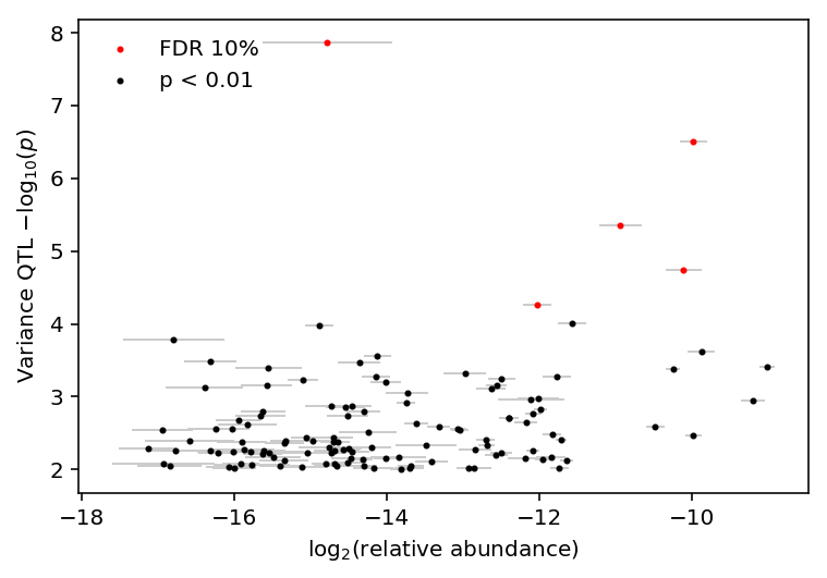
Investigate whether variance QTL \(p\)-values are correlated with relative abundance.
variance_qtls = qtls['zinb/variance'][0]
thresh_pass = variance_qtls['p_beta'] < 1e-2
var_qtl_abundance, var_qtl_stats = abundance.align(variance_qtls[thresh_pass].set_index('gene'), axis='index', join='inner')
fdr_pass = var_qtl_stats['fdr_pass']
Count how many variance QTLs have \(p < 10^{-2}\)
thresh_pass.sum()
121
plt.clf()
plt.errorbar(x=var_qtl_abundance.mean(axis=1), y=-np.log10(var_qtl_stats['p_beta']), xerr=var_qtl_abundance.std(axis=1), fmt='none', label=None, lw=1, ecolor='.8', zorder=-1)
plt.scatter(x=var_qtl_abundance[fdr_pass].mean(axis=1), y=-np.log10(var_qtl_stats[fdr_pass]['p_beta']), c='r', s=4, label='FDR 10%')
plt.scatter(x=var_qtl_abundance[~fdr_pass].mean(axis=1), y=-np.log10(var_qtl_stats[~fdr_pass]['p_beta']), c='k', s=4, label='p < 0.01')
plt.legend(loc='upper left', frameon=False)
plt.xlabel('$\log_2(\mathrm{relative\ abundance})$')
_ = plt.ylabel('Variance QTL $-\log_{10}(p)$')
Make sure our effect sizes match qtltools.
variance = qtls['zinb/variance'][1]
Xv, Yv = extract_qtl_gene_pair(variance_qtls[thresh_pass], variance, dosages='/scratch/midway2/aksarkar/singlecell/scqtl-mapping/yri-120-dosages.vcf.gz')
Cv = pd.read_table('/project2/mstephens/aksarkar/projects/singlecell-qtl/data/scqtl-mapping/variance-covars.txt', index_col=0)
Cv = Cv.align(Xv, axis='columns', join='inner')[0]
my_var_qtl_stats = replication_tests(Xv, Yv, Cv)
my_var_qtl_stats.merge(variance_qtls, on='gene').apply(lambda x: abs(x['beta_x'] - x['beta_y']), axis=1).describe()
count       121
mean     0.0904
std       0.105
min     0.00246
25%      0.0255
50%      0.0601
75%       0.132
max       0.867
dtype: float64
Look at the gene with max difference in estimated effect size.
my_var_qtl_stats.iloc[my_var_qtl_stats.merge(variance_qtls, on='gene').apply(lambda x: abs(x['beta_x'] - x['beta_y']), axis=1).idxmax()]
beta               20.3
gene    ENSG00000079102
p                 0.157
se                 14.4
Name: 116, dtype: object
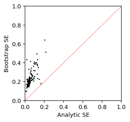
Estimate standard errors via the bootstrap.
var_qtl_stats['bootstrap_se'] = bootstrap_se(Xv, Yv, Cv)
var_qtl_stats['se'] = my_var_qtl_stats.set_index('gene')['se']
Investigate whether analytic SEs are reasonable:
var_qtl_stats['se'].describe()
count       121
mean       0.18
std         1.3
min     0.00832
25%      0.0311
50%      0.0447
75%       0.078
max        14.4
Name: se, dtype: float64
var_qtl_stats['bootstrap_se'].describe()
count      121
mean      1.22
std       9.12
min     0.0995
25%      0.178
50%      0.217
75%      0.285
max        100
Name: bootstrap_se, dtype: float64
Plot analytic SEs against bootstrap SEs.
plt.clf()
plt.gcf().set_size_inches(3, 3)
plt.scatter(var_qtl_stats['se'], var_qtl_stats['bootstrap_se'], s=1, c='k')
plt.plot([0, 1], [0, 1], c='r', ls=':', lw=1)
plt.xlim([0, 1])
plt.ylim([0, 1])
plt.xlabel('Analytic SE')
_ = plt.ylabel('Bootstrap SE')
Compute \(z\)-scores using the bootstrap SEs.
var_qtl_stats['z'] = var_qtl_stats['beta'] / var_qtl_stats['bootstrap_se']
Compute a \(z\)-score from the estimated effect size and the \(p\)-value.
var_qtl_stats['isf_z'] = np.sign(var_qtl_stats['beta']) * np.sqrt(st.chi2(1).isf(var_qtl_stats['p_nominal']))
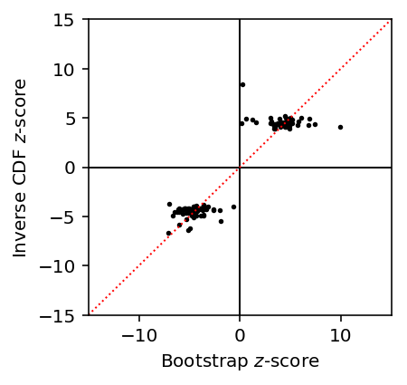
Plot bootstrap \(z\)-scores against inverse-transformed \(z\)-scores.
plt.clf()
plt.gcf().set_size_inches(3, 3)
plt.scatter(var_qtl_stats['z'], var_qtl_stats['isf_z'], s=3, c='k')
plt.axhline(y=0, c='k', lw=1)
plt.axvline(x=0, c='k', lw=1)
plt.plot([-15, 15], [-15, 15], c='r', ls=':', lw=1)
plt.xlim([-15, 15])
plt.ylim([-15, 15])
plt.xlabel('Bootstrap $z$-score')
_ = plt.ylabel('Inverse CDF $z$-score')
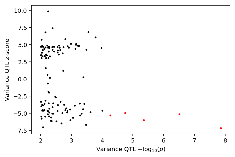
Investigate whether \(z\)-scores based on bootstrap SEs agree with permutation \(p\)-values.
plt.clf()
plt.scatter(-np.log10(var_qtl_stats[fdr_pass]['p_beta']), var_qtl_stats[fdr_pass]['z'], c='r', label='FDR 10%', s=4)
plt.scatter(-np.log10(var_qtl_stats[~fdr_pass]['p_beta']), var_qtl_stats[~fdr_pass]['z'], c='k', label='p < 0.01', s=4)
plt.xlabel('Variance QTL $-\log_{10}(p)$')
plt.ylabel('Variance QTL $z$-score')
Text(0,0.5,'Variance QTL $z$-score')
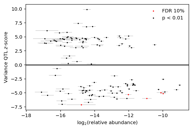
Investigate whether variance QTL \(z\)-scores are correlated with relative abundance.
var_qtl_abundance = var_qtl_abundance.align(var_qtl_stats, axis='index', join='inner')[0]
plt.clf()
plt.errorbar(x=var_qtl_abundance.mean(axis=1), y=var_qtl_stats['z'], xerr=var_qtl_abundance.std(axis=1), fmt='none', label=None, lw=1, ecolor='.8', zorder=1)
plt.scatter(x=var_qtl_abundance[fdr_pass].mean(axis=1), y=var_qtl_stats[fdr_pass]['z'], c='r', s=2, label='FDR 10%', zorder=2)
plt.scatter(x=var_qtl_abundance[~fdr_pass].mean(axis=1), y=var_qtl_stats[~fdr_pass]['z'], c='k', s=2, label='p < 0.01', zorder=2)
plt.legend(frameon=False)
plt.axhline(y=0, c='k')
plt.xlabel('$\log_2(\mathrm{relative\ abundance})$')
_ = plt.ylabel('Variance QTL $z$-score')
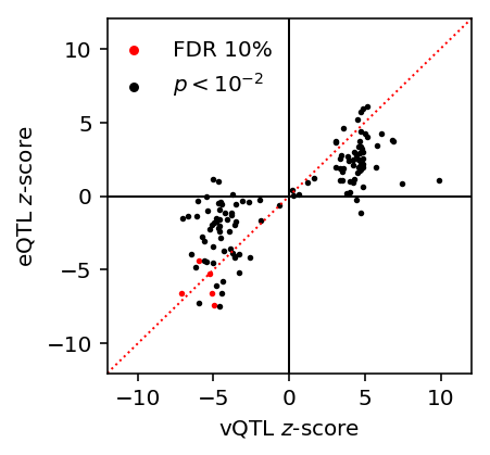
Investigate whether variance QTL \(z\)-scores are correlated with mean QTL \(z\)-scores.
Xm, Ym = extract_qtl_gene_pair(variance_qtls[thresh_pass], qtls['zinb/mean'][1], dosages='/scratch/midway2/aksarkar/singlecell/scqtl-mapping/yri-120-dosages.vcf.gz')
Cm = covars[1]
Cm = Cm.align(Xm, axis='columns', join='inner')[0]
var_qtl_stats['mean_beta'] = replication_tests(Xm, Ym, Cm).set_index('gene')['beta']
var_qtl_stats['mean_z'] = var_qtl_stats['mean_beta'] / bootstrap_se(Xm, Ym, Cm)
Plot variance QTL \(z\)-scores against pooled QTL \(z\)-scores.
lim = [-12, 12]
plt.clf()
plt.gcf().set_size_inches(3, 3)
plt.plot(lim, lim, c='r', ls=':', lw=1)
plt.scatter(var_qtl_stats[fdr_pass]['z'], var_qtl_stats[fdr_pass]['mean_z'], c='r', s=3, label='FDR 10%')
plt.scatter(var_qtl_stats[~fdr_pass]['z'], var_qtl_stats[~fdr_pass]['mean_z'], c='k', s=3, label='$p < 10^{-2}$')
plt.legend(frameon=False, markerscale=2, loc=(-.01, .75))
plt.axhline(y=0, c='k', lw=1)
plt.axvline(x=0, c='k', lw=1)
plt.xlim(lim)
plt.ylim(lim)
plt.xlabel('vQTL $z$-score')
_ = plt.ylabel('eQTL $z$-score')
Compute the same in the other direction.
mean_qtl_stats = qtls['zinb/mean'][0]
mean_qtl_stats = mean_qtl_stats[mean_qtl_stats['fdr_pass']].copy()
X, Y = extract_qtl_gene_pair(mean_qtl_stats, qtls['zinb/mean'][1], dosages='/scratch/midway2/aksarkar/singlecell/scqtl-mapping/yri-120-dosages.vcf.gz')
z = mean_qtl_stats.set_index('gene')['beta'] / bootstrap_se(X, Y, Cm)

X, Y = extract_qtl_gene_pair(mean_qtl_stats, qtls['zinb/variance'][1], dosages='/scratch/midway2/aksarkar/singlecell/scqtl-mapping/yri-120-dosages.vcf.gz')
vz = replication_tests(X, Y, Cv).set_index('gene')['beta'] / bootstrap_se(X, Y, Cv)

Xb, Yb = extract_qtl_gene_pair(mean_qtl_stats, qtls['bulk'][1], dosages='/scratch/midway2/aksarkar/singlecell/scqtl-mapping/yri-120-dosages.vcf.gz')
Cb = pd.read_table('/project2/mstephens/aksarkar/projects/singlecell-qtl/data/scqtl-mapping/bulk-covars.txt', sep=r'\s+', engine='python')
Cb = Cb.align(Xb, axis='columns', join='inner')[0]
bulk_z = replication_tests(Xb, Yb, Cb).set_index('gene')['beta'] / bootstrap_se(Xb, Yb, Cb)

mean_qtl_stats = mean_qtl_stats.set_index('gene')
mean_qtl_stats['z'] = z
mean_qtl_stats['var_z'] = vz
mean_qtl_stats['bulk_z'] = bulk_z
mean_qtl_stats['var_fdr_pass'] = mean_qtl_stats.index.isin(fdr_pass[fdr_pass].index)
Plot mean vs. variance \(z\)-scores at eQTL SNP-gene pairs.
lim = [-12, 12]
plt.clf()
plt.gcf().set_size_inches(3, 3)
plt.plot(lim, lim, c='r', ls=':', lw=1)
plt.scatter(mean_qtl_stats.loc[mean_qtl_stats['var_fdr_pass'], 'var_z'],
            mean_qtl_stats.loc[mean_qtl_stats['var_fdr_pass'], 'z'], c='r',
            s=3, label='vQTL')
plt.scatter(mean_qtl_stats.loc[~mean_qtl_stats['var_fdr_pass'], 'var_z'],
            mean_qtl_stats.loc[~mean_qtl_stats['var_fdr_pass'], 'z'], c='k',
            s=3, label='Not vQTL')
plt.legend(frameon=False, markerscale=2, loc=(-.01, .75))
plt.axhline(y=0, c='k', lw=1)
plt.axvline(x=0, c='k', lw=1)
plt.xlim(lim)
plt.ylim(lim)
plt.xlabel('vQTL $z$-score')
_ = plt.ylabel('eQTL $z$-score')
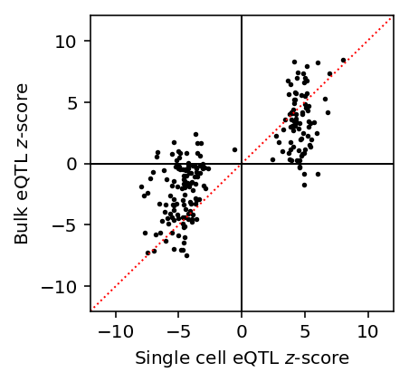
Plot single cell eQTL \(z\)-scores against bulk eQTL \(z\)-scores.
lim = [-12, 12]
plt.clf()
plt.gcf().set_size_inches(3, 3)
plt.plot(lim, lim, c='r', ls=':', lw=1)
plt.scatter(mean_qtl_stats['z'], mean_qtl_stats['bulk_z'], c='k', s=3)
plt.axhline(y=0, c='k', lw=1)
plt.axvline(x=0, c='k', lw=1)
plt.xlim(lim)
plt.ylim(lim)
plt.xlabel('Single cell eQTL $z$-score')
_ = plt.ylabel('Bulk eQTL $z$-score')
Joint distribution of summary statistics
Read the nominal summary statistics.
stats = {x: pd.read_table('/project2/mstephens/aksarkar/projects/singlecell-qtl/data/power/{}.txt.gz'.format(x), index_col=0)
         for x in ('bulk', 'mean', 'variance')}
Compute \(z\)-scores.
for k in stats:
  stats[k]['z'] = stats[k]['beta'] / stats[k]['se']
Munge the bulk gene names.
stats['bulk']['gene'] = [x.split('.')[0] for x in stats['bulk']['gene']]
Munge the index names.
for k in stats:
  stats[k].index.name = 'id'
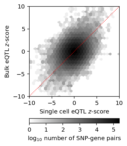
Plot the joint distribution of bulk/mean \(z\)-scores.
J = stats['mean'].reset_index().merge(stats['bulk'].reset_index(), on=['id', 'gene'])[['z_x', 'z_y']]
plt.clf()
plt.gcf().set_size_inches(3, 4)
plt.hexbin(J['z_x'], J['z_y'], gridsize=30, extent=[-10, 10, -10, 10], bins='log', cmap=colorcet.cm['gray_r'])
plt.gca().set_aspect('equal')
plt.xlim(-10, 10)
plt.ylim(-10, 10)
plt.plot(plt.ylim(), plt.ylim(), c='r', ls=':', lw=1)
cb = plt.colorbar(orientation='horizontal')
cb.set_label('$\log_{10}$ number of SNP-gene pairs')
plt.xlabel('Single cell eQTL $z$-score')
plt.ylabel('Bulk eQTL $z$-score')
plt.tight_layout()
Plot single cell eQTL \(z\)-scores against bulk eQTL \(z\)-scores.
J = (stats['mean']
     .reset_index()
     .merge(qtls['mean'][0][qtls['mean'][0]['fdr_pass']], on=['id', 'gene'])
     [['id', 'gene', 'beta_x', 'se']]
     .merge(stats['bulk'].reset_index(), on=['id', 'gene']))
lim = [-12, 12]
plt.clf()
plt.gcf().set_size_inches(3, 3)
plt.plot(lim, lim, c='r', ls=':', lw=1)
plt.scatter(J['beta_x'] / J['se_x'], J['beta'] / J['se_y'], c='k', s=3)
plt.axhline(y=0, c='k', lw=1)
plt.axvline(x=0, c='k', lw=1)
plt.xlim(lim)
plt.ylim(lim)
plt.xlabel('Single cell eQTL $z$-score')
_ = plt.ylabel('Bulk eQTL $z$-score')
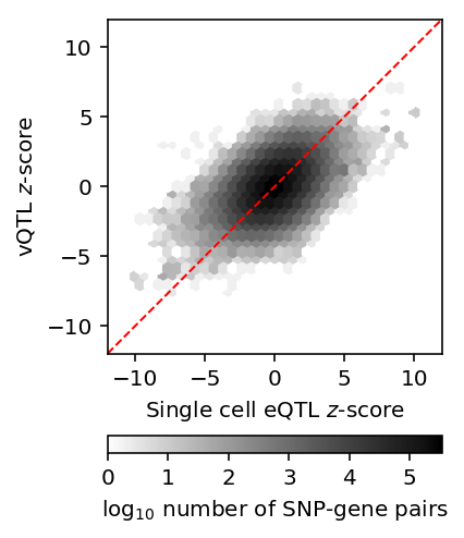
Plot the joint distribution of mean/variance \(z\)-scores.
J = stats['mean'].reset_index().merge(stats['variance'].reset_index(), on=['id', 'gene'])[['z_x', 'z_y']]
plt.clf()
plt.gcf().set_size_inches(3, 4)
plt.hexbin(J['z_x'], J['z_y'], gridsize=30, extent=[-10, 10, -10, 10], bins='log', cmap=colorcet.cm['gray_r'])
plt.gca().set_aspect('equal')
plt.xlim(-12, 12)
plt.ylim(-12, 12)
plt.plot(plt.ylim(), plt.ylim(), c='r', ls='--', lw=1)
cb = plt.colorbar(orientation='horizontal')
cb.set_label('$\log_{10}$ number of SNP-gene pairs')
plt.xlabel('Single cell eQTL $z$-score')
plt.ylabel('vQTL $z$-score')
plt.tight_layout()
Plot the significant SC vQTL \(z\)-scores, and their corresponding \(z\)-score for the mean.
J = (stats['variance']
     .reset_index()
     .merge(qtls['variance'][0][qtls['variance'][0]['fdr_pass']], on=['id', 'gene'])
     [['id', 'gene', 'beta_x', 'se']]
     .merge(stats['mean'].reset_index(), on=['id', 'gene']))
lim = [-12, 12]
plt.clf()
plt.gcf().set_size_inches(3, 3)
plt.plot(lim, lim, c='r', ls=':', lw=1)
plt.scatter(J['beta_x'] / J['se_x'], J['beta'] / J['se_y'], c='k', s=3)
plt.axhline(y=0, c='k', lw=1)
plt.axvline(x=0, c='k', lw=1)
plt.xlim(lim)
plt.ylim(lim)
plt.xlabel('vQTL $z$-score')
_ = plt.ylabel('eQTL $z$-score')
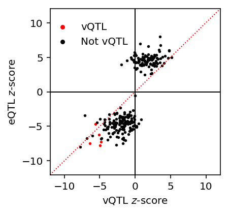
Plot the significant SC eQTL \(z\)-scores, and their corresponding \(z\)-score for the mean.
J = (stats['mean']
     .reset_index()
     .merge(qtls['mean'][0][qtls['mean'][0]['fdr_pass']], on=['id', 'gene'])
     [['id', 'gene', 'beta_x', 'se']]
     .merge(stats['variance'].reset_index(), on=['id', 'gene'])
     .merge(qtls['variance'][0], on=['id', 'gene'], suffixes=['_y', '_z'], how='left')
     .fillna(False))
lim = [-12, 12]
plt.clf()
plt.gcf().set_size_inches(3, 3)
plt.plot(lim, lim, c='r', ls=':', lw=1)
colors = {True: 'r', False: 'k'}
labels = {True: 'vQTL', False: 'not vQTL'}
for k, g in J.groupby('fdr_pass'):
  plt.scatter(g['beta_x'] / g['se_x'], g['beta_y'] / g['se_y'], c=colors[k], s=3, label=labels[k])
plt.legend(frameon=False, markerscale=2, handletextpad=0, loc=(-.01, .75))
plt.axhline(y=0, c='k', lw=1)
plt.axvline(x=0, c='k', lw=1)
plt.xlim(lim)
plt.ylim(lim)
plt.ylabel('vQTL $z$-score')
_ = plt.xlabel('eQTL $z$-score')
Predicting mean QTLs from variance QTLs
As we change the threshold for calling mean (variance) QTLs, track the precision and recall of variance (mean) QTLs.
plt.clf()
plt.gcf().set_size_inches(3, 3)
Y, P = qtls['mean'][0]['fdr_pass'].align(qtls['variance'][0]['p_beta'].dropna(), join='inner')
p, r, _ = sklearn.metrics.precision_recall_curve(Y.astype(int), -np.log(P))
auprc_mean_var = sklearn.metrics.average_precision_score(Y.astype(int), -np.log(P))
plt.plot(r[::10], p[::10], lw=1, c='k', label='Variance')
Y, P = qtls['variance'][0]['fdr_pass'].align(qtls['mean'][0]['p_beta'].dropna(), join='inner')
p, r, _ = sklearn.metrics.precision_recall_curve(Y.astype(int), -np.log(P))
auprc_var_mean = sklearn.metrics.average_precision_score(Y.astype(int), -np.log(P))
plt.plot(r[::10], p[::10], lw=1, c='r', label='Mean')
plt.legend(frameon=False)
plt.xlabel('Recall of QTLs at FDR 10%')
_ = plt.ylabel('Precision of QTLs at FDR 10%')
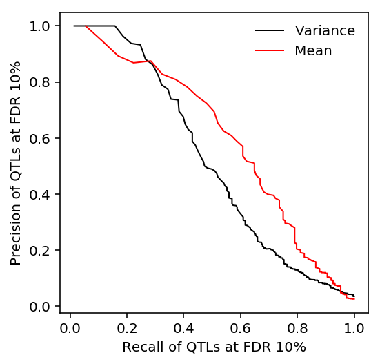
Tabulate the AUPRC.
auprc_mean_var, auprc_var_mean
(0.5212419583724434, 0.6044457996921822)
Track sensitivity and specificity of mean QTLs.
plt.clf()
plt.gcf().set_size_inches(3, 3)
Y, P = qtls['mean'][0]['fdr_pass'].align(qtls['variance'][0]['p_beta'].dropna(), join='inner')
fpr, tpr, _ = sklearn.metrics.roc_curve(Y.astype(int), -np.log(P))
auroc_mean_var = sklearn.metrics.roc_auc_score(Y.astype(int), -np.log(P))
plt.plot(fpr[::10], tpr[::10], lw=1, c='k', label='Variance')
Y, P = qtls['variance'][0]['fdr_pass'].align(qtls['mean'][0]['p_beta'].dropna(), join='inner')
fpr, tpr, _ = sklearn.metrics.roc_curve(Y.astype(int), -np.log(P))
auroc_var_mean = sklearn.metrics.roc_auc_score(Y.astype(int), -np.log(P))
plt.plot(fpr[::10], tpr[::10], lw=1, c='r', label='Mean')
plt.legend(frameon=False)
plt.xlabel('False positive rate of QTLs at FDR 10%')
_ = plt.ylabel('True positive rate of QTLs at FDR 10%')
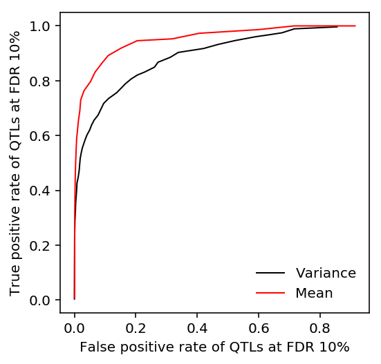
Tabulate the AUROC.
auroc_mean_var, auroc_var_mean
(0.8968614143396433, 0.9555166119581557)
Find the threshold at which 90% of eQTLs are recovered.
Y, P = qtls['variance'][0].set_index('gene')['fdr_pass'].align(qtls['mean'][0].set_index('gene')['p_beta'].dropna(), join='inner')
fpr, tpr, thresh = sklearn.metrics.roc_curve(Y.astype(int), -np.log(P))
np.exp(-thresh[np.where(tpr <= 0.9)].min())
0.05222859999999999
Find the vQTLs which are not predictive of eQTLs.
true_negatives = Y[np.logical_and(Y, -np.log(P) < thresh[np.where(tpr <= 0.9)].min())].to_frame().merge(gene_info, left_index=True, right_index=True)[['name']]
true_negatives
name
gene
ENSG00000122574      WIPF3
ENSG00000112367       FIG4
ENSG00000121481       RNF2
ENSG00000214194  LINC00998
ENSG00000133935    C14orf1
ENSG00000243725       TTC4
ENSG00000132849      INADL
ENSG00000171130   ATP6V0E2
ENSG00000129518       EAPP
ENSG00000182400   TRAPPC6B
ENSG00000182117      NOP10
ENSG00000068024      HDAC4
ENSG00000169714       CNBP
ENSG00000133030      MPRIP
ENSG00000108528   SLC25A11