Cell-to-cell variation analysis: cells not detected as expressed

Background and some observations
Set up
Prepare data
Drop-out rate descriptives
Explore the role of drop-outs
Compare non-detection rates between individuals
Non-detection rate p-value and fold change
Differential non-detectoin rate and CV
Non-detection, fold change, CV: NA19098 vs. NA19101
Pluripotency genes
Session information

Last updated: 2016-07-08

Code version: f3271c626c586079652907b55fa357b6f569fd26

Background and some observations

Non-detection rate descriptives: We found that the median of non-detected cells rate is 26% across the three individuals and ranges between 21 to 30% between the three individuals.
Non-detection rate and Mean, Var, CV: Expectedly, gene abundance and variance were both associated with percent of non-detected cells; even genes with as low as 10 percent of non-detected cells were restricted in the dynamic range of abudance levels. Gene coefficient of variation was not correlated with percent of non-detected genes (Spearman’s correlation = .04) across the three individuals. Further analysis indicated that when including only cells with less than 50 percent of undetected cells, the gene CV decreases as a concave function of abundance, a commonly observed pattern in bulk RNA-seq data and in scRNA-seq when undetected cells are included in the analysis.
Compare non-detection rates: 1,958 genes were found to have significant differences in non-detection rates between the three individuals at false discovery rate less than .01.
Individual difference in non-detection rate and gene abundance: We found no correlation between p-values of tests comparing gene mean abundance and p-values of tests comparing non-detection rate, for all three pairiwse between-individual comparisons. The results also held when we investigated the correlation between fold change and p-value of tests comparing non-detection rate between indivdiuals. Furthermore, we evaluated genes with absolute log2 fold change greater than 1, 1.5, and 2 in the pairwise comparison tests, most genes with our nominated fold change difference were found to not have a significant difference in the proportion of non-detected cells.

*Note: I don’t trust the differential expression analysis results here. Over 95% of the genes in the overall F-test were to be significant at FDR < .01; same results were found for two of the pairwise comparisons (NA19098-NA19101, NA19098-NA19239). When looking at the fold change of gene expression, I found only a very small portion of the genes with log2 fold change more than 2; NA19098-NA19101: 5 genes, NA19098-NA19239: 4 genes, and NA19101-NA19101: 2 genes.

Note: An interesting observation when computing fold change suggests that on average gene abundance levels of NA19239 > NA19101> NA19098

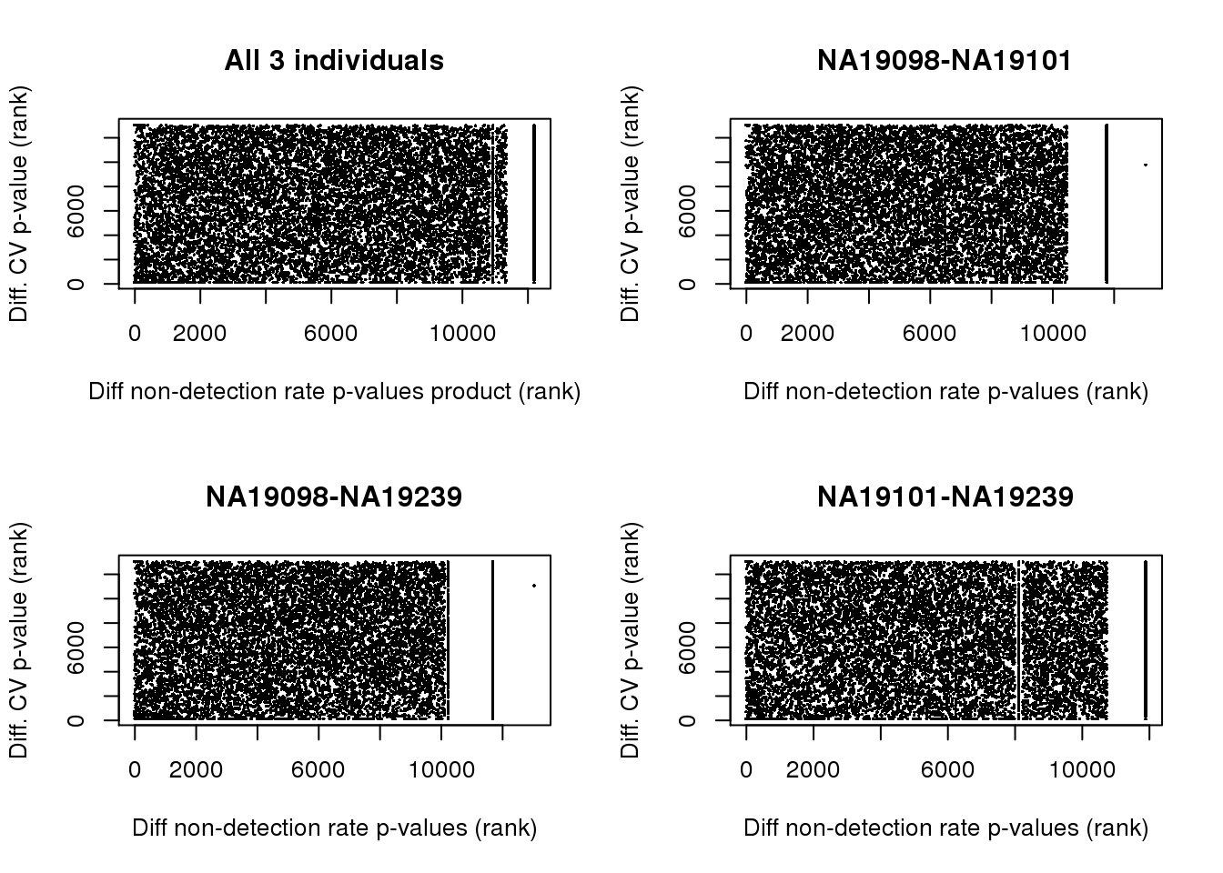
Non-detection rate and adjusted CV of the expressed cells: Similar to results with gene abundance, we found no correlation between individual differences in non-detection rate and adjusted CV. At FDR < .01, of the 679 genes with differential adjusted CV of the expressed cells, only 69 genes were found to have significant difference also in proportion of undetected cells in at least one pair of between individual comparisons.

Set up

library("dplyr")
library("limma")
library("edgeR")
library("ggplot2")
library("scales")
library("grid")
theme_set(theme_bw(base_size = 12))
source("functions.R")
library("Humanzee")
library("cowplot")
library("MASS")
library("matrixStats")
source("../code/cv-functions.r")
source("../code/plotting-functions.R")
library("mygene")
library("aod")

Prepare data

We import molecule counts before standardizing and transformation and also log2-transformed counts after batch-correction. Biological variation analysis of the individuals is performed on the batch-corrected and log2-transformed counts.

# Import filtered annotations
anno_filter <- read.table("../data/annotation-filter.txt", 
                      header = TRUE,
                      stringsAsFactors = FALSE)

# Import filtered molecule counts
molecules_filter <- read.table("../data/molecules-filter.txt",
                               header = TRUE, stringsAsFactors = FALSE)
stopifnot(NROW(anno_filter) == NCOL(molecules_filter))

# Import final processed molecule counts of endogeneous genes
molecules_final <- read.table("../data/molecules-final.txt", 
                             header = TRUE, stringsAsFactors = FALSE)
stopifnot(NROW(anno_filter) == NCOL(molecules_final))

# Import gene symbols
gene_symbols <- read.table(file = "../data/gene-info.txt", sep = "\t",
                           header = TRUE, stringsAsFactors = FALSE, quote = "")

# Import cell-cycle gene list
cell_cycle_genes <- read.table("../data/cellcyclegenes.txt",
                               header = TRUE, sep = "\t",
                               stringsAsFactors = FALSE)

# Import pluripotency gene list

pluripotency_genes <- read.table("../data/pluripotency-genes.txt",
                               header = TRUE, sep = "\t",
                               stringsAsFactors = FALSE)$To

Load gene CVs computed over all cells (link1), CV computed only over the expressed cells (link2), and differential CV results when including only the expressed cells (link3).

load("../data/cv-all-cells.rda")
load("../data/cv-expressed-cells.rda")
load("../data/permuted-pval-expressed-set1.rda")

Compute a matrix of 0’s and 1’s indicating non-detected and detected cells, respectively.

molecules_expressed <- molecules_filter
molecules_expressed[which(molecules_filter > 0 , arr.ind = TRUE)] <- 1
molecules_expressed <- as.matrix((molecules_expressed))

Take the gene subset included in the final data.

genes_included <- Reduce(intersect,
                         list(rownames(molecules_final),
                             rownames(expressed_cv$NA19098),
                             names(perm_pval_set1)) )

molecules_filter_subset <- molecules_filter[
  which(rownames(molecules_filter) %in% genes_included), ]

molecules_final_subset <- molecules_final[
  which(rownames(molecules_final) %in% genes_included), ]

molecules_expressed_subset <- molecules_expressed[
  which(rownames(molecules_expressed) %in% genes_included), ]

molecules_final_expressed_subset <- molecules_final_subset*molecules_expressed_subset
molecules_final_expressed_subset[which(molecules_expressed_subset == 0, arr.ind = TRUE)] <- NA

permuted_pval_subset <- perm_pval_set1[which(names(perm_pval_set1) %in% genes_included)]
names(permuted_pval_subset) <- names(perm_pval_set1)[which(names(perm_pval_set1) %in% genes_included)]

expressed_cv_subset <- lapply(expressed_cv, function(x)
  x[which(rownames(x) %in% genes_included), ] )
names(expressed_cv_subset) <- names(expressed_cv)

expressed_dm_subset <- expressed_dm[which(rownames(expressed_dm) %in% genes_included), , ] 

dim(molecules_final_subset)

[1] 13043   564

dim(molecules_expressed_subset)

[1] 13043   564

all.equal(rownames(expressed_cv_subset$NA19098), 
          rownames(molecules_final_expressed_subset) )

[1] TRUE

all.equal(names(permuted_pval_subset), 
          rownames(molecules_expressed_subset) )

[1] TRUE

Drop-out rate descriptives

Compute drop-out rates.

drop_out <- lapply(unique(anno_filter$individual), function(ind) {
  temp_df <- molecules_filter_subset[,anno_filter$individual == ind]
  zero_df <- array(0, dim = dim(temp_df))
  rownames(zero_df) <- rownames(temp_df)
  zero_df[which(temp_df == 0, arr.ind = TRUE)] <- 1
  zero_count <- rowMeans(zero_df)
  return(zero_count)
})  
names(drop_out) <- unique(anno_filter$individual)
drop_out$all <- rowMeans(as.matrix(molecules_filter_subset) == 0)

summary(drop_out$NA19098)

   Min. 1st Qu.  Median    Mean 3rd Qu.    Max. 
0.00000 0.02113 0.21130 0.32060 0.59860 0.99300

summary(drop_out$NA19101)

   Min. 1st Qu.  Median    Mean 3rd Qu.    Max. 
0.00000 0.04975 0.29350 0.36500 0.66170 0.99500

summary(drop_out$NA19239)

   Min. 1st Qu.  Median    Mean 3rd Qu.    Max. 
0.00000 0.02715 0.25340 0.35060 0.65610 0.99550

summary(drop_out$all)

   Min. 1st Qu.  Median    Mean 3rd Qu.    Max. 
0.00000 0.03723 0.26060 0.34820 0.64540 0.93090

Histogram of drop-out percents.

par(mfrow = c(2,2))
for (i in 1:4) {
h1 <- hist(drop_out[[i]], breaks = seq(0,1, by = .1), 
           plot = FALSE)
h1$density <- h1$counts/sum(h1$counts)*100
plot(h1, ylab = "Percent",
         xlab = "Proportion of non-detected cells",
         main = names(drop_out)[i], 
     freq=FALSE)
}

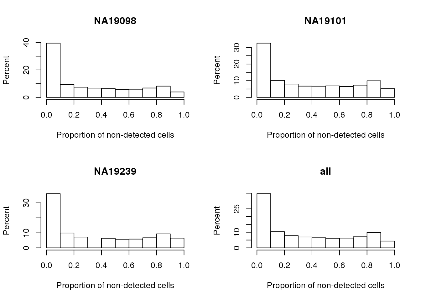
Proportion of genes with 50 percent or more undetected cells.

sapply(drop_out, function(x) mean(x>=.5))

  NA19098   NA19101   NA19239       all 
0.3091313 0.3592732 0.3378057 0.3384957

Explore the role of drop-outs

NA19098, expressed cells

par(mfrow = c(2,2))
plot(y = log10(expressed_cv_subset$NA19098$expr_mean),
     x = drop_out$NA19098,
     xlab = "Percent of drop-outs",
     ylab = "log10 mean expression",
     pch = 16, cex =.3)
lines(lowess( expressed_cv_subset$NA19098$expr_mean ~ drop_out$NA19098),
      col = "red")
plot(y = log10(expressed_cv_subset$NA19098$expr_var),
     x = drop_out$NA19098,
     xlab = "Percent of drop-outs",
     ylab = "log10 variance of expression",
     pch = 16, cex =.3)
lines(lowess( log10(expressed_cv_subset$NA19098$expr_var) ~ drop_out$NA19098),
      col = "red")
plot(y = expressed_cv_subset$NA19098$expr_cv,
     x = drop_out$NA19098,
     xlab = "Percent of drop-outs",
     ylab = "CV",
     pch = 16, cex =.3)
lines(lowess( expressed_cv_subset$NA19098$expr_cv ~ drop_out$NA19098),
      col = "red")
plot(y = expressed_dm_subset$NA19098,
     x = drop_out$NA19098,
     xlab = "Percent of drop-outs",
     ylab = "Corrected CV",
     pch = 16, cex =.3)
lines(lowess( expressed_dm_subset$NA19098 ~ drop_out$NA19098),
      col = "red")
title(main = "Expressed cells, NA19098", outer = TRUE, line = -1)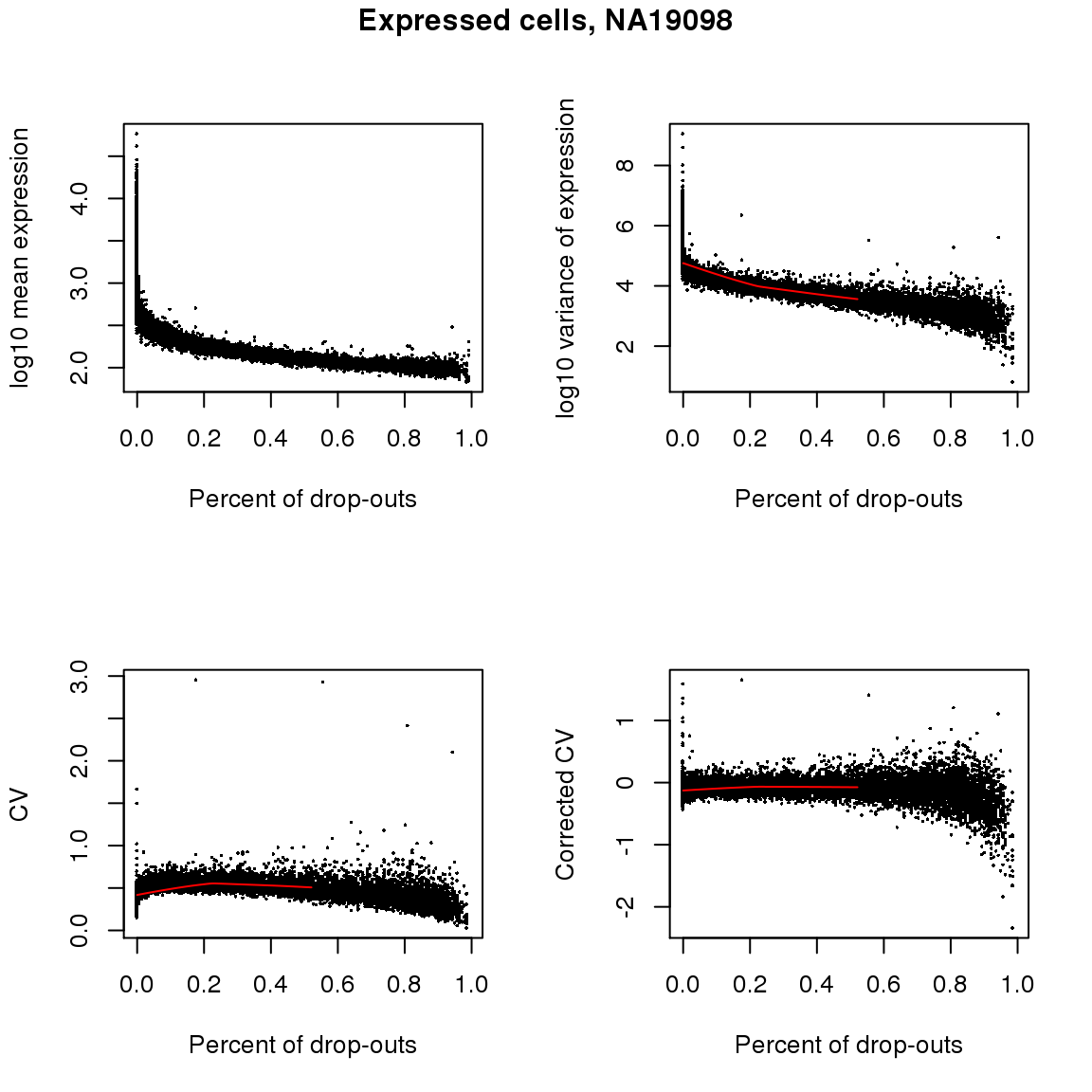

All individuals, expressed cells

par(mfrow = c(2,2))
# abundance
plot(y = log10(expressed_cv_subset$all$expr_mean),
     x = drop_out$all,
     xlab = "Percent of drop-outs",
     ylab = "log10 mean expression",
     pch = 16, cex =.3)
lines(lowess( log10(expressed_cv_subset$all$expr_mean) ~ drop_out$all),
      col = "red")
# variance
plot(y = log10(expressed_cv_subset$all$expr_var),
     x = drop_out$all,
     xlab = "Percent of drop-outs",
     ylab = "log10 variance of expression",
     pch = 16, cex =.3)
lines(lowess( log10(expressed_cv_subset$all$expr_var) ~ drop_out$all),
      col = "red")
# CV
plot(y = expressed_cv_subset$all$expr_cv,
     x = drop_out$all,
     xlab = "Percent of drop-outs",
     ylab = "CV",
     pch = 16, cex =.3)
lines(lowess( expressed_cv_subset$all$expr_cv ~ drop_out$all),
      col = "red")
title(main = "All 3 individuals", outer = TRUE, line = -1)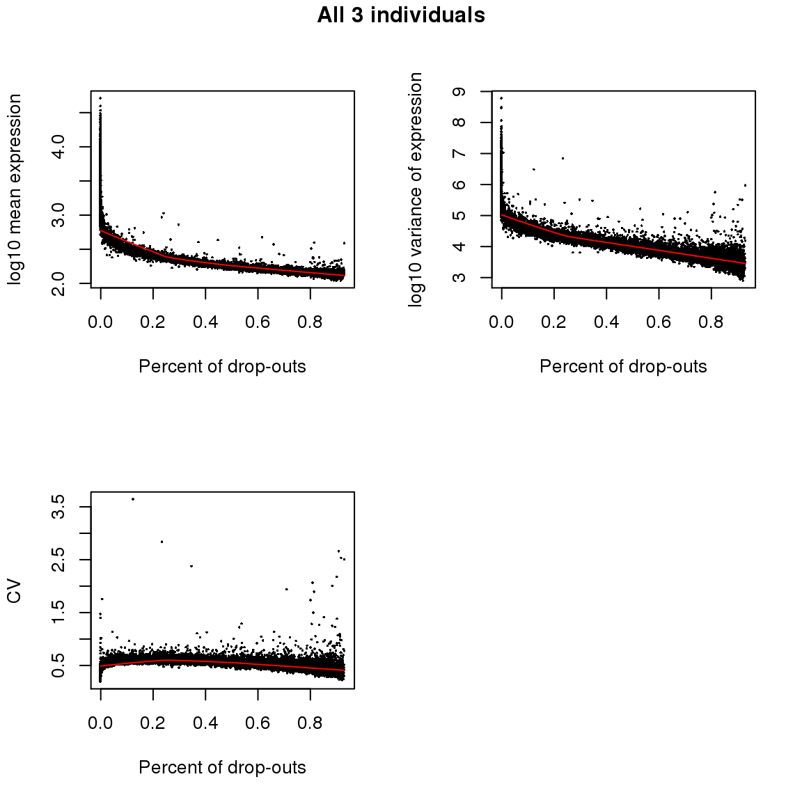

CV and mean plus drop-out rates.

par(mfrow = c(2,2))
plot(y = expressed_cv_subset$NA19098$expr_cv,
     x = log10(expressed_cv_subset$NA19098$expr_mean),
     cex = .9, col = alpha("grey40", .8), lwd = .6,
     xlab = "log10 gene mean abundance",
     ylab = "CV",
     main = "Expressed cells, NA19098",
     xlim = c(1,5), ylim = c(0,2.5))
points(y = expressed_cv_subset$NA19098$expr_cv,
       x = log10(expressed_cv_subset$NA19098$expr_mean), 
       col = rev(RColorBrewer::brewer.pal(10, "RdYlBu"))[
                cut(drop_out$NA19098, breaks = seq(0, 1, by = .1),
                     include.lowest = TRUE)], 
       cex = .6, pch = 16)


plot(y = expressed_cv_subset$all$expr_cv,
     x = log10(expressed_cv_subset$all$expr_mean),
     cex = .9, col = alpha("grey40", .8), lwd = .6,
     xlab = "log10 gene mean abundance",
     ylab = "CV",
     main = "Expressed cells, All 3 individuals",
     xlim = c(1,5), ylim = c(0,2.5))
points(y = expressed_cv_subset$all$expr_cv,
       x = log10(expressed_cv_subset$all$expr_mean), 
       col = rev(RColorBrewer::brewer.pal(10, "RdYlBu"))[
                cut(drop_out$all, breaks = seq(0, 1, by = .1),
                     include.lowest = TRUE)], 
       cex = .6, pch = 16)


plot(y = expressed_dm_subset$NA19098,
     x = log10(expressed_cv_subset$NA19098$expr_mean),
     cex = .9, col = alpha("grey40", .8), lwd = .6,
     xlab = "log10 gene mean abundance",
     ylab = "Adjusted CV",
     main = "Expressed cells, NA19098",
     xlim = c(1,5))
points(y = expressed_dm_subset$NA19098,
       x = log10(expressed_cv_subset$NA19098$expr_mean), 
       col = rev(RColorBrewer::brewer.pal(10, "RdYlBu"))[
                cut(drop_out$NA19098, breaks = seq(0, 1, by = .1),
                     include.lowest = TRUE)], 
       cex = .6, pch = 16)

plot(1:10, pch = 15, cex = 2, axes = F, xlab = "", ylab = "",
     col = rev(RColorBrewer::brewer.pal(10, "RdYlBu")), xlim = c(0, 13))
text(labels = levels(cut(drop_out$NA19098, breaks = seq(0, 1, by = .1),
                     include.lowest = TRUE)),
     y = 1:10, x = 1:10 + 2, cex = .7)
title(main = "drop-out rate")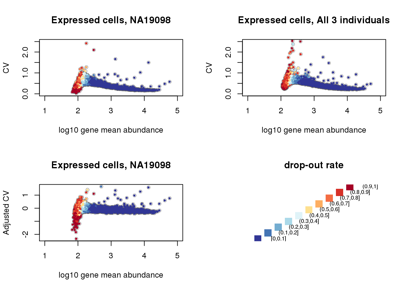

Compare non-detection rates between individuals

Fisher’s exact test for between individual comparisons. For some genes, we observed no undetected cells, a scenario that calls for Fisher’s exact test instead of Chi-square test or logistic regression.

file_name <- "../data/sig-test-zeros.rda"
if (file.exists(file_name)) {
  load(file_name)
} else {
  ind <- factor(anno_filter$individual,
              levels = unique(anno_filter$individual),
              labels = unique(anno_filter$individual) )
  fit_zero <- do.call(rbind,
      lapply(1:NROW(molecules_expressed_subset), function(ii) {
#      lapply(1:100, function(ii) {
          tab <- table(molecules_expressed_subset[ii, ], ind)
          if (dim(tab)[1] == 1) {
             if (as.numeric(rownames(tab)) == 1) {
               tab <- rbind(rep(0,3), tab)
               rownames(tab) <- c(0,1)
             } else {
               tab <- rbind(rep(1,3), tab)
               rownames(tab) <- c(0,1)
             }
          }
          pval <- lapply(rev(1:dim(tab)[2]),
                         function(i) {
                              fisher.test(tab[,-i])$p.value                 
                         })
          names(pval) <- sapply(rev(1:dim(tab)[2]), 
                               function(i) {
                                 paste(colnames(tab[,-i])[1],
                                      colnames(tab[,-i])[2],
                                      sep = "-") })
          df <- data.frame(
                do.call(cbind, pval),
                    row.names = rownames(molecules_expressed_subset)[ii] ) 
          colnames(df) <- names(pval)
          return(df)
  }) )
  fit_zero_qval <- do.call(cbind,
    lapply(1:3, function(i) {
    stats::p.adjust(fit_zero[,i], method = "fdr")
  }))
  colnames(fit_zero_qval) <- colnames(fit_zero)
  
  save(fit_zero, fit_zero_qval, file = file_name)
}

par(mfrow = c(2,2))
for (i in 1:3) {
  hist(fit_zero[,i],
       main = colnames(fit_zero)[i],
       xlab = "p-value")
}
title(main = "p-value histogram", outer = TRUE, line = -1)

# genes with almost 1 p-value
table(rowSums(fit_zero > .999))


   0    1    2    3 
8865 2188  282 1708

par(mfrow = c(2,2))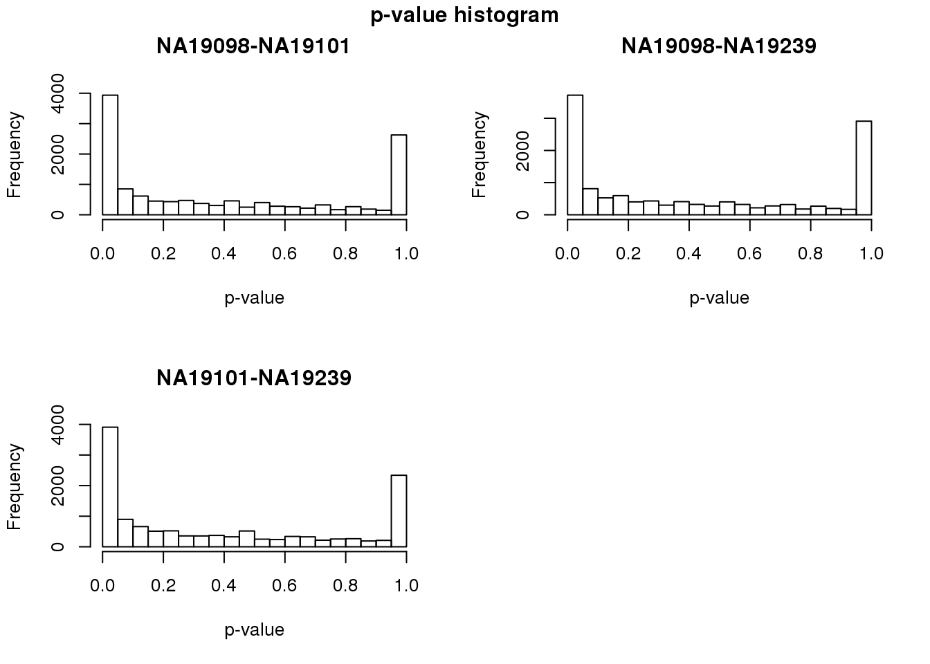

for (i in 1:3) {
  plot(ecdf(fit_zero[,i]),
       main = colnames(fit_zero)[i],
       xlab = "p-value",
       axes = F)
  axis(1); axis(2)
}
title(main = "p-value empirical distribution function", outer = TRUE, line = -1)


par(mfrow = c(2,2))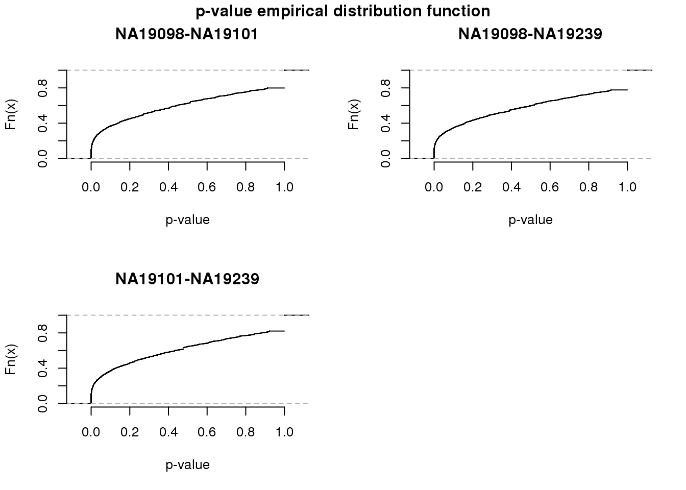

for (i in 1:3) {
  plot(ecdf(fit_zero_qval[,i]),
       main = colnames(fit_zero_qval)[i],
       xlab = "q-value",
       axes = F)
  axis(1); axis(2)
}
title(main = "q-value empirical distribution function", outer = TRUE, line = -1)

table(rowSums(fit_zero_qval < .01))


   0    1    2    3 
9877 1746 1347   73

library(VennDiagram)
library(gridExtra)
genes <- rownames(molecules_expressed_subset)
overlap_list <- lapply(1:3, function(i)
      genes[ which( fit_zero_qval[ ,i] < .01 ) ] )
names(overlap_list) <- colnames(fit_zero_qval)

grid.arrange(gTree(children = venn.diagram(overlap_list,filename = NULL,
                          category.names = names(overlap_list),
                          name = "q-val < .01")) )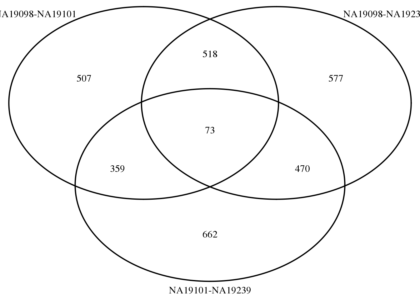

Non-detection rate p-value and fold change

log2fc <- data.frame(
  NA19098_NA19101 = rowMeans(molecules_final_expressed_subset[,anno_filter$individual == "NA19098"], na.rm = TRUE) - rowMeans(molecules_final_expressed_subset[,anno_filter$individual == "NA19101"], na.rm = TRUE),
  NA19098_NA19239 = rowMeans(molecules_final_expressed_subset[,anno_filter$individual == "NA19098"], na.rm = TRUE) - rowMeans(molecules_final_expressed_subset[,anno_filter$individual == "NA19239"], na.rm = TRUE),
  NA19101_NA19239 = rowMeans(molecules_final_expressed_subset[,anno_filter$individual == "NA19101"], na.rm = TRUE) - rowMeans(molecules_final_expressed_subset[,anno_filter$individual == "NA19239"], na.rm = TRUE) )


par(mfrow = c(2,2))
plot(rank(fit_zero$`NA19098-NA19101`), 
     rank(log2fc$NA19098_NA19101),
     pch = 16, cex = .3,
     xlab = "Differential non-detection rate p-value (rank)",
     ylab = "log2 fold change (rank)",
     main = "NA19098-NA19101") 
plot(rank(fit_zero$`NA19098-NA19239`), 
     rank(log2fc$NA19098_NA19239),
     pch = 16, cex = .3,
     xlab = "Differential non-detection rate p-value (rank)",
     ylab = "log2 fold change (rank)",
     main = "NA19098-NA19239") 
plot(rank(fit_zero$`NA19101-NA19239`), 
     rank(log2fc$NA19101_NA19239),
     pch = 16, cex = .3,
     xlab = "Differential non-detection rate p-value (rank)",
     ylab = "log2 fold change (rank)",
     main = "NA19101-NA19239")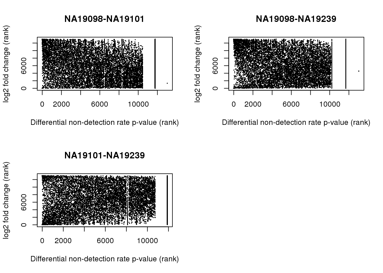

print("abs. log2 FC > 1")

[1] "abs. log2 FC > 1"

sapply(log2fc, function(x) sum(abs(x) > 1))

NA19098_NA19101 NA19098_NA19239 NA19101_NA19239 
            178             164              32

library(VennDiagram)
library(gridExtra)
genes <- rownames(molecules_final_subset)
overlap_list <- lapply(1:3, function(i)
  list(diffNonDetection = genes[which(fit_zero_qval[,i] < .01)],
       diffAbundance = genes[ which( abs(log2fc[[i]]) > 1) ]) )
names(overlap_list) <- colnames(fit_zero_qval)

grid.arrange(gTree(children = venn.diagram(overlap_list[[1]],filename = NULL,
                          category.names = names(overlap_list[[1]]))),
            gTree(children = venn.diagram(overlap_list[[2]],filename = NULL,
                          category.names = names(overlap_list[[1]]))),
            gTree(children = venn.diagram(overlap_list[[3]],filename = NULL,
                          category.names = names(overlap_list[[3]]))),
      ncol = 2)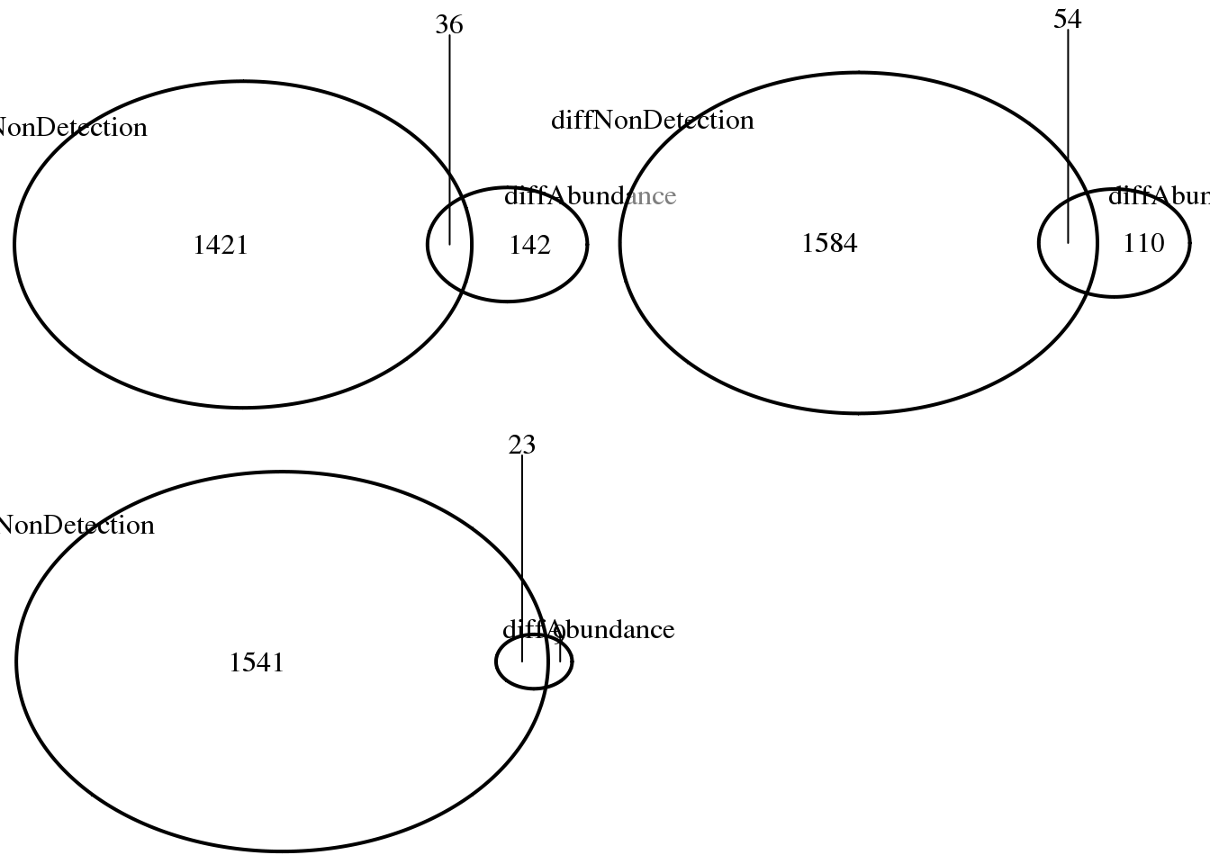

print("abs. log2 FC > 1.5")

[1] "abs. log2 FC > 1.5"

sapply(log2fc, function(x) sum(abs(x) > 1.5))

NA19098_NA19101 NA19098_NA19239 NA19101_NA19239 
             12              12              10

genes <- rownames(molecules_final_subset)
overlap_list <- lapply(1:3, function(i)
  list(diffNonDetection = genes[which(fit_zero_qval[,i] < .01)],
       diffAbundance = genes[ which( abs(log2fc[[i]]) > 1.5) ]) )
names(overlap_list) <- colnames(fit_zero_qval)

grid.arrange(gTree(children = venn.diagram(overlap_list[[1]],filename = NULL,
                          category.names = names(overlap_list[[1]]))),
            gTree(children = venn.diagram(overlap_list[[2]],filename = NULL,
                          category.names = names(overlap_list[[1]]))),
            gTree(children = venn.diagram(overlap_list[[3]],filename = NULL,
                          category.names = names(overlap_list[[3]]))),
      ncol = 2)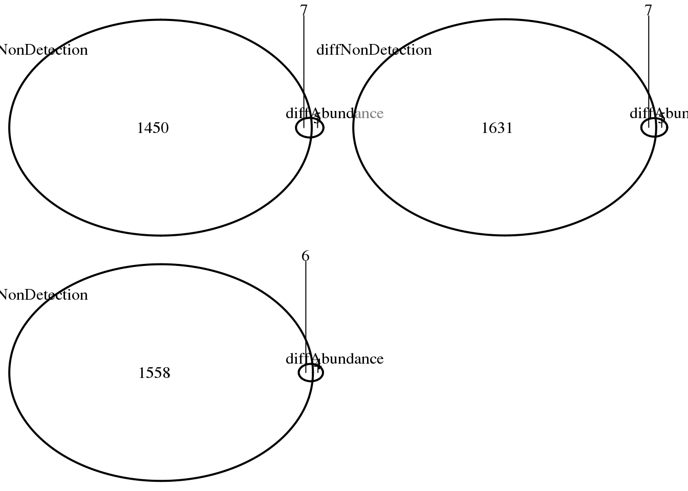

print("abs. log2 FC > 2")

[1] "abs. log2 FC > 2"

sapply(log2fc, function(x) sum(abs(x) > 2))

NA19098_NA19101 NA19098_NA19239 NA19101_NA19239 
              5               6               2

genes <- rownames(molecules_final_subset)
overlap_list <- lapply(1:3, function(i)
  list(diffNonDetection = genes[which(fit_zero_qval[,i] < .01)],
       diffAbundance = genes[ which( abs(log2fc[[i]]) > 2) ]) )
names(overlap_list) <- colnames(fit_zero_qval)

grid.arrange(gTree(children = venn.diagram(overlap_list[[1]],filename = NULL,
                          category.names = names(overlap_list[[1]]))),
            gTree(children = venn.diagram(overlap_list[[2]],filename = NULL,
                          category.names = names(overlap_list[[1]]))),
            gTree(children = venn.diagram(overlap_list[[3]],filename = NULL,
                          category.names = names(overlap_list[[3]]))),
      ncol = 2)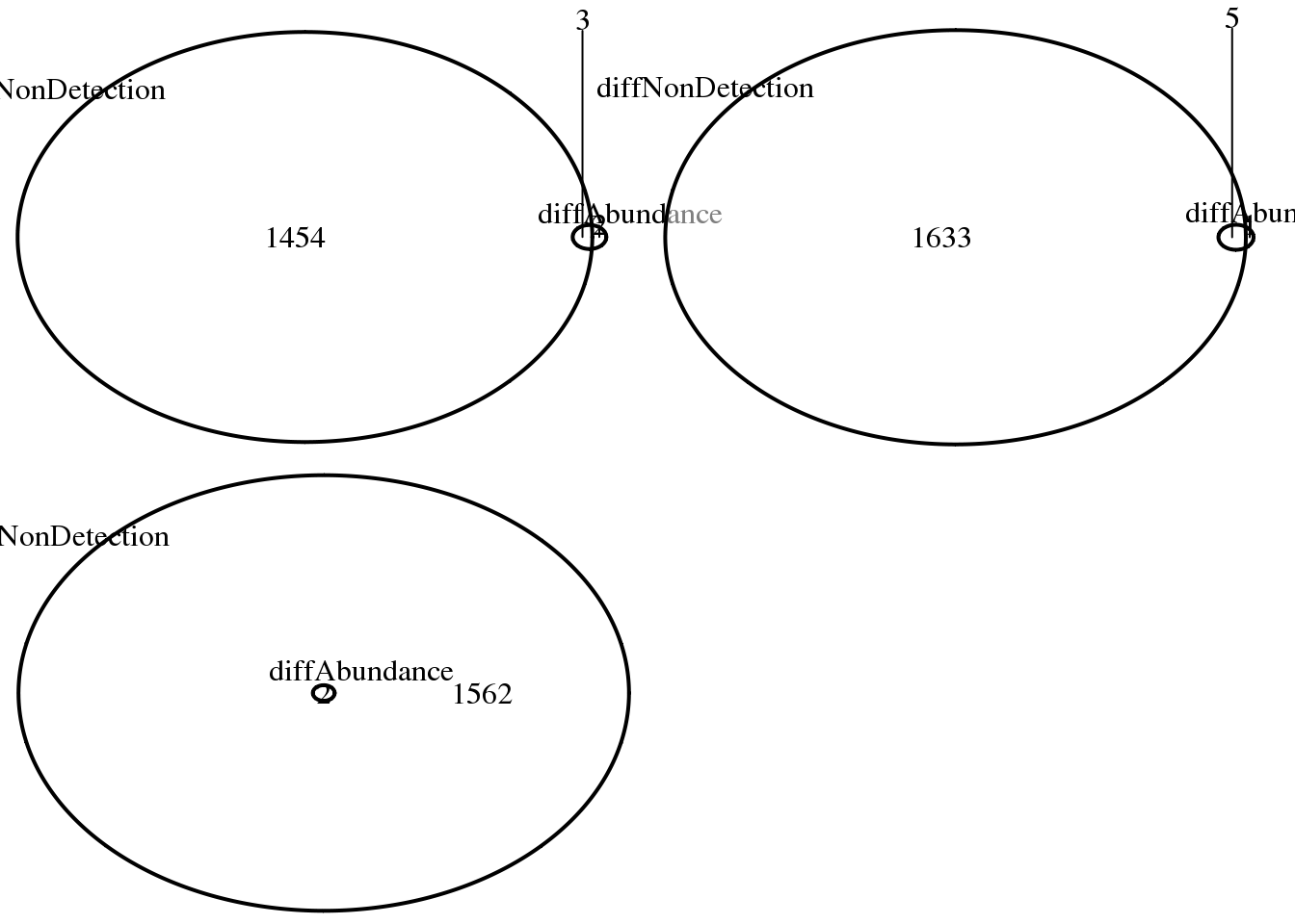

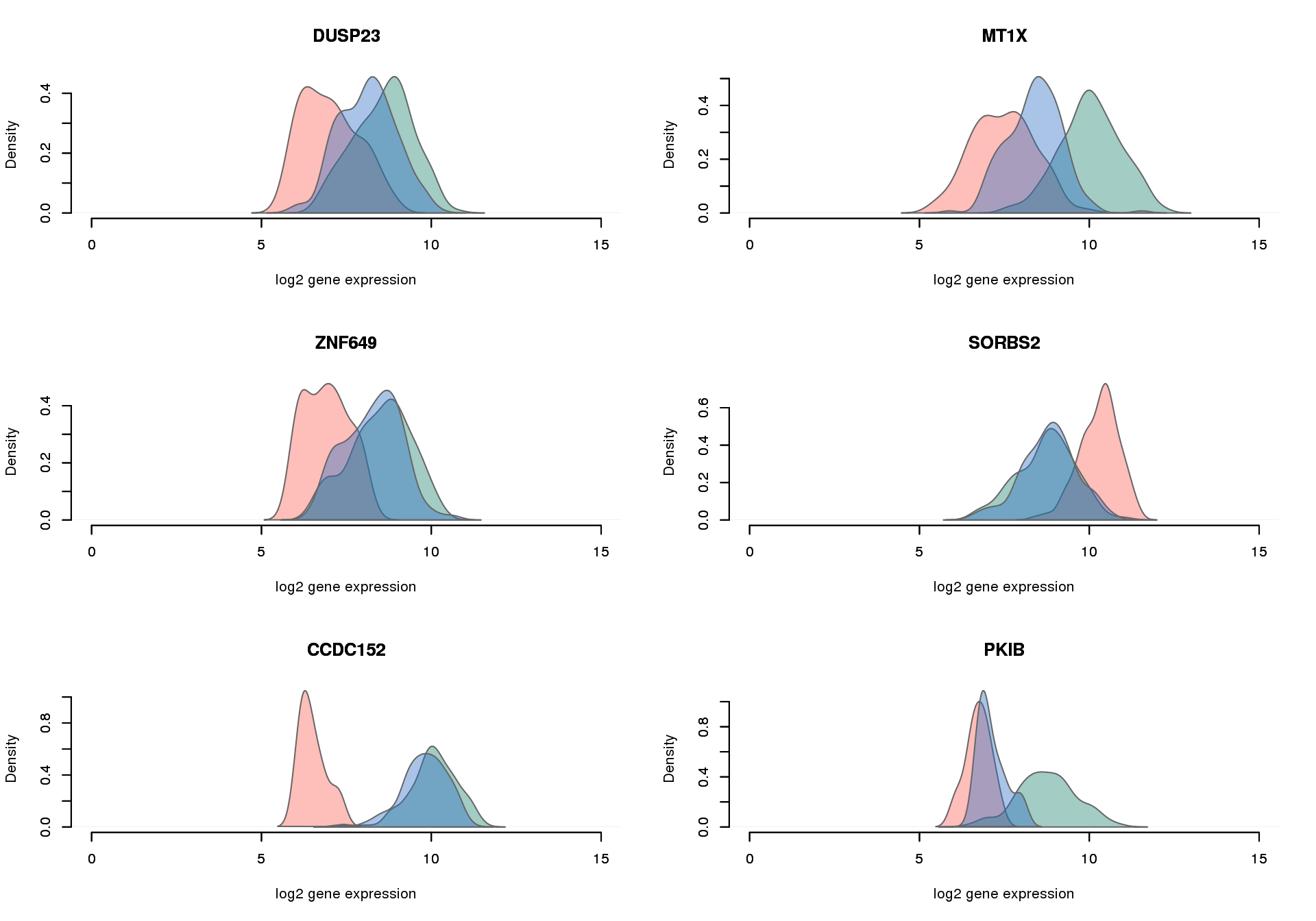
NA19098 vs. NA19101: diff non-detection,log2FC > 1.5

# genes with the largest difference in non-detection rates
gene_elect <- intersect(
  rownames(fit_zero)[which(fit_zero_qval[,1] < .01)],
  rownames(log2fc)[ which(abs(log2fc$NA19098_NA19101) > 1.5) ] )
                         

par(mfrow = c(3,2))
for (i in 1:6) {
  plot_density_overlay(
    molecules = molecules_final_expressed_subset,
    annotation = anno_filter,
    which_gene = gene_elect[i], 
    labels = "",
    xlims = c(0,15), ylims = NULL,
    gene_symbols = gene_symbols)
}

Differential non-detectoin rate and CV

par(mfrow = c(2,2))
plot(x = rank(matrixStats::rowProds(as.matrix(fit_zero), na.rm =TRUE)),
     y = rank(permuted_pval_subset),
     pch = 16, cex = .3,
     ylab ="Diff. CV p-value (rank)",
     xlab = "Diff non-detection rate p-values product (rank)",
     main = "All 3 individuals")
for (i in 1:3) {
plot(x = rank(fit_zero[,i]),
     y = rank(permuted_pval_subset),
     pch = 16, cex = .3,
     ylab ="Diff. CV p-value (rank)",
     xlab = "Diff non-detection rate p-values (rank)",
     main = colnames(fit_zero)[i] )
}

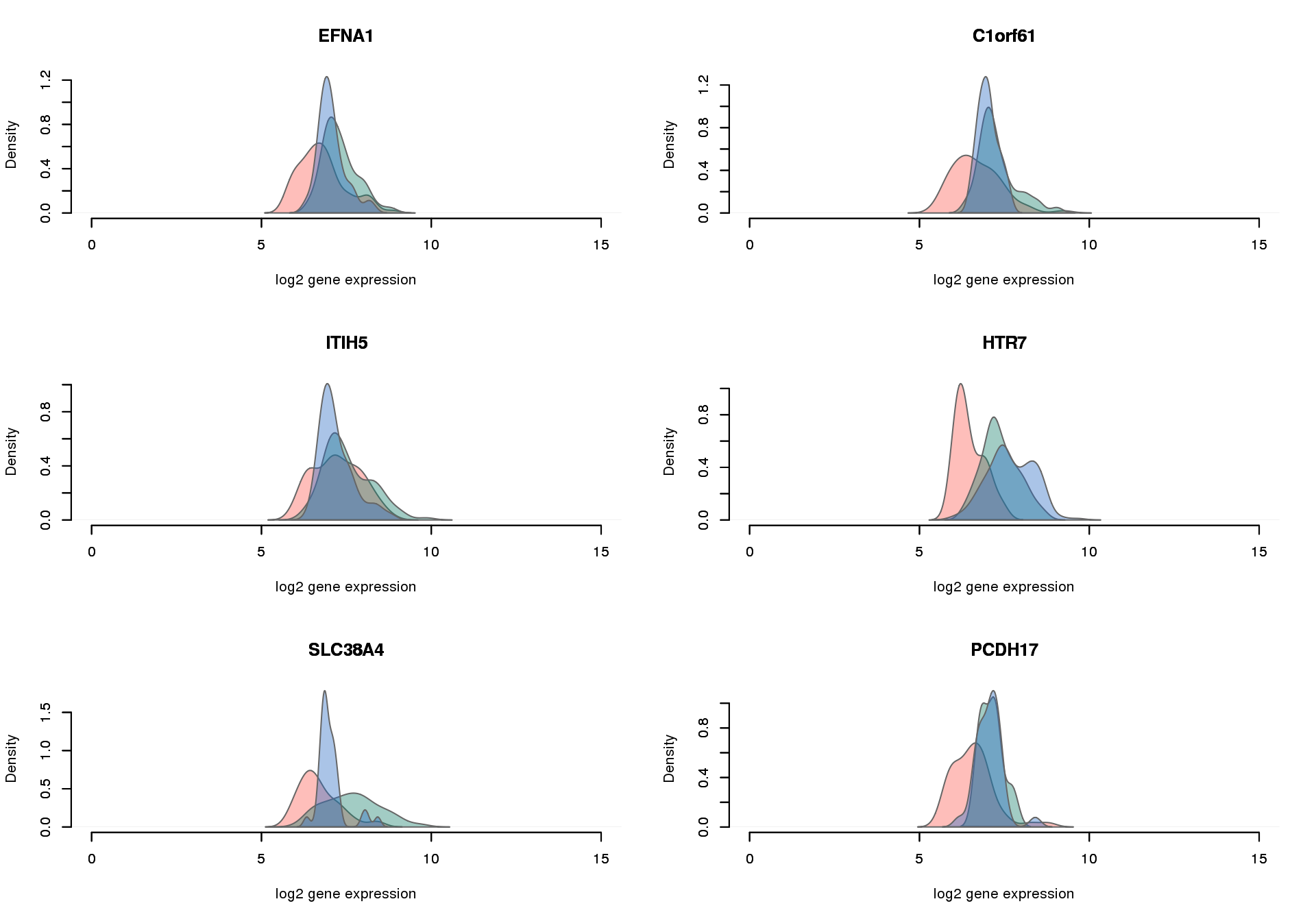
Overlap of genes with at least one significant pairwise difference in proportion of detected genes, and genes with significant differential CV.

# subset expression data of genes that were included
# in the significance testing
rownames(fit_zero_qval) <- rownames(fit_zero)

library(VennDiagram)
library(gridExtra)
overlap_list_diff <- list(
   diffCV = names(permuted_pval_subset)[which(permuted_pval_subset == 0)],
   diffNonDetection = rownames(fit_zero_qval)[
     which(rowSums(fit_zero_qval < .01, na.rm = TRUE) > 1)
   ])  

grid.arrange(gTree(children = venn.diagram(overlap_list_diff,filename = NULL,
                          category.names = names(overlap_list_diff),
                          name = "Diff. CV & non-detected rate")))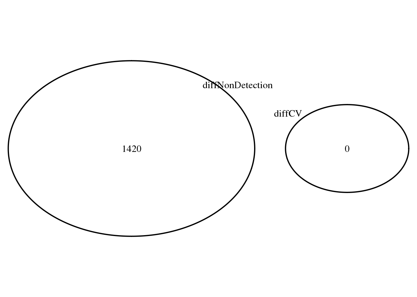

# genes with the largest difference in non-detection rates
gene_elect <- intersect(
  rownames(fit_zero)[which(rowSums(fit_zero_qval < .01, na.rm = TRUE) == 1)],
  rownames(log2fc)[ which(permuted_pval_subset < .01) ] )
                         
par(mfrow = c(3,2))
for (i in 1:6) {
  plot_density_overlay(
    molecules = molecules_final_expressed_subset,
    annotation = anno_filter,
    which_gene = gene_elect[i], 
    labels = "",
    xlims = c(0,15), ylims = NULL,
    gene_symbols = gene_symbols)
}

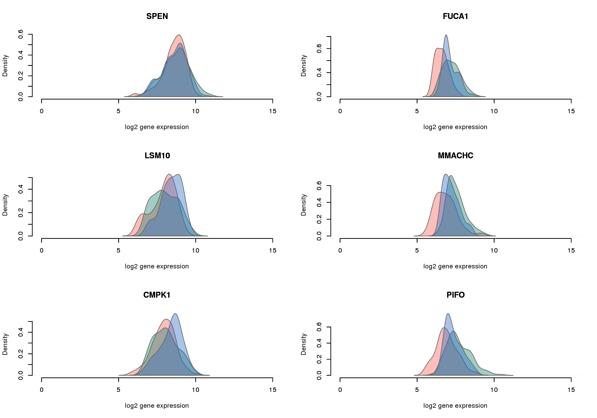
Overlap of genes with significant difference in proportion of undetected genes between all three pairs and overlap of genes with significant differential CV genes.

# subset expression data of genes that were included
# in the significance testing
rownames(fit_zero_qval) <- rownames(fit_zero)

library(VennDiagram)
library(gridExtra)
overlap_list_diff <- list(
   diffCV = names(permuted_pval_subset)[which(permuted_pval_subset == 0)],
   diffNonDetection = rownames(fit_zero_qval)[
     which(rowSums(fit_zero_qval < .01, na.rm = TRUE) == 3)
   ])  

grid.arrange(gTree(children = venn.diagram(overlap_list_diff,filename = NULL,
                          category.names = names(overlap_list_diff),
                          name = "Diff. CV & non-detected rate")))

# genes with the largest difference in non-detection rates
gene_elect <- intersect(
  rownames(fit_zero)[which(rowSums(fit_zero_qval < .01, na.rm = TRUE) == 3)],
  rownames(log2fc)[ which(permuted_pval_subset < .01) ] )
                         
par(mfrow = c(3,2))
for (i in 1:6) {
  plot_density_overlay(
    molecules = molecules_final_expressed_subset,
    annotation = anno_filter,
    which_gene = gene_elect[i], 
    labels = "",
    xlims = c(0,15), ylims = NULL,
    gene_symbols = gene_symbols)
}

Non-detection, fold change, CV: NA19098 vs. NA19101

# subset expression data of genes that were included
# in the significance testing
rownames(fit_zero_qval) <- rownames(fit_zero)

library(VennDiagram)
library(gridExtra)
overlap_list_diff <- list(
   difflog2FC = rownames(log2fc)[which(abs(log2fc$NA19098_NA19101) > 1)],
   diffCV = names(permuted_pval_subset)[which(permuted_pval_subset == 0)],
   diffNonDetection = rownames(fit_zero_qval)[
     which(fit_zero_qval[,1] < .01) ] )  

grid.arrange(gTree(children = venn.diagram(overlap_list_diff,filename = NULL,
                          category.names = names(overlap_list_diff))))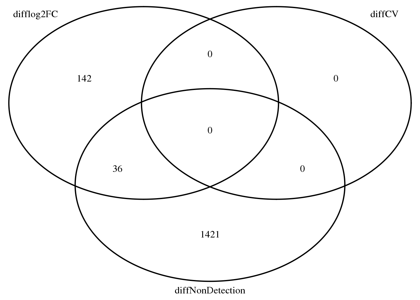

Pluripotency genes

pluri <- rownames(fit_zero)[which(rownames(fit_zero) %in% pluripotency_genes)]
symbol <- gene_symbols$external_gene_name[match(pluri, gene_symbols$ensembl_gene_id)]

zero_prop <- do.call(cbind,
    lapply(unique(anno_filter$individual), function(ind) {
        rowMeans(molecules_expressed_subset[, anno_filter$individual == ind] == 0,
                 na.rm = TRUE)
      }) )
colnames(zero_prop) <- unique(anno_filter$individual)
names(zero_prop) <- unique(anno_filter$individual)      

summary_table <- data.frame(
  gene_symbo = symbol, 
  diffCVpval = permuted_pval_subset[which(names(permuted_pval_subset) %in% pluripotency_genes)] < .01,
  fit_zero_qval[which(rownames(fit_zero) %in% pluripotency_genes), ] < .01,
  round(log2fc[which(rownames(log2fc) %in% pluripotency_genes), ], digits = 2),
  round(zero_prop[which(rownames(log2fc) %in% pluripotency_genes), ], digits = 2),
  stringsAsFactors = FALSE)


# The two significant CV genes


#DNMT3B
table(molecules_expressed_subset[which( rownames(molecules_expressed_subset) %in% "ENSG00000088305"), ])


  1 
564

summary(unlist(molecules_final_expressed_subset[which( rownames(molecules_final_expressed_subset) %in% "ENSG00000088305"), ]) )

   Min. 1st Qu.  Median    Mean 3rd Qu.    Max. 
  10.80   12.03   12.35   12.36   12.71   13.72

# N66A1
table(molecules_expressed_subset[which( rownames(molecules_expressed_subset) %in% "ENSG00000148200"), ])


  1 
564

summary(unlist(molecules_final_expressed_subset[which( rownames(molecules_final_expressed_subset) %in% "ENSG00000148200"), ]) )

   Min. 1st Qu.  Median    Mean 3rd Qu.    Max. 
  10.23   11.21   11.50   11.50   11.79   12.91

# NANOG
table(molecules_expressed_subset[which( rownames(molecules_expressed_subset) %in% "ENSG00000111704"), ])


  0   1 
125 439

summary(unlist(molecules_final_expressed_subset[which( rownames(molecules_final_expressed_subset) %in% "ENSG00000111704"), ]) )

   Min. 1st Qu.  Median    Mean 3rd Qu.    Max.    NA's 
  5.977   7.184   7.678   7.784   8.368  10.550     125

#ZFP42
table(molecules_expressed_subset[which( rownames(molecules_expressed_subset) %in% "ENSG00000179059"), ])


  0   1 
  1 563

summary(unlist(molecules_final_expressed_subset[which( rownames(molecules_final_expressed_subset) %in% "ENSG00000179059"), ]) )

   Min. 1st Qu.  Median    Mean 3rd Qu.    Max.    NA's 
  6.556   9.722  10.380  10.220  10.810  11.770       1

kable(summary_table)

	gene_symbo	diffCVpval	NA19098.NA19101	NA19098.NA19239	NA19101.NA19239	NA19098_NA19101	NA19098_NA19239	NA19101_NA19239	NA19098	NA19101	NA19239
ENSG00000187140	FOXD3	FALSE	FALSE	TRUE	FALSE	-0.49	-0.10	0.39	0.30	0.46	0.53
ENSG00000156574	NODAL	FALSE	TRUE	FALSE	FALSE	-0.15	-0.49	-0.34	0.82	0.96	0.93
ENSG00000171794	UTF1	FALSE	FALSE	TRUE	TRUE	-0.68	-0.51	0.17	0.89	0.89	0.98
ENSG00000184344	GDF3	FALSE	FALSE	TRUE	TRUE	-0.37	-0.10	0.26	0.18	0.29	0.45
ENSG00000111704	NANOG	FALSE	FALSE	FALSE	TRUE	-0.84	-0.25	0.58	0.18	0.13	0.33
ENSG00000102554	KLF5	TRUE	FALSE	TRUE	FALSE	-0.91	-0.41	0.50	0.99	0.96	0.87
ENSG00000088305	DNMT3B	TRUE	FALSE	FALSE	FALSE	-0.51	0.31	0.81	0.00	0.00	0.00
ENSG00000101115	SALL4	TRUE	FALSE	FALSE	FALSE	-0.33	-0.09	0.24	0.00	0.00	0.00
ENSG00000163530	DPPA2	TRUE	TRUE	TRUE	FALSE	-0.60	-0.41	0.19	0.67	0.84	0.89
ENSG00000121570	DPPA4	FALSE	FALSE	FALSE	FALSE	-0.13	-0.11	0.03	0.00	0.00	0.00
ENSG00000181449	SOX2	FALSE	FALSE	FALSE	FALSE	-0.44	-0.32	0.12	0.00	0.00	0.00
ENSG00000179059	ZFP42	FALSE	FALSE	FALSE	FALSE	-1.37	-1.34	0.03	0.01	0.00	0.00
ENSG00000164362	TERT	FALSE	FALSE	FALSE	FALSE	-0.42	-0.18	0.24	0.62	0.54	0.58
ENSG00000204531	POU5F1	FALSE	FALSE	FALSE	FALSE	-0.60	-0.29	0.31	0.00	0.00	0.00
ENSG00000124762	CDKN1A	FALSE	FALSE	TRUE	TRUE	-0.38	-0.32	0.06	0.59	0.60	0.91
ENSG00000203909	DPPA5	FALSE	FALSE	TRUE	TRUE	-0.54	-0.14	0.39	0.66	0.65	0.99
ENSG00000128567	PODXL	FALSE	FALSE	FALSE	FALSE	-0.46	0.10	0.56	0.00	0.00	0.00
ENSG00000136997	MYC	FALSE	FALSE	FALSE	TRUE	-1.07	-0.03	1.04	0.04	0.03	0.11
ENSG00000136826	KLF4	TRUE	FALSE	FALSE	FALSE	-0.70	-0.78	-0.09	0.96	0.93	0.86
ENSG00000148200	NR6A1	FALSE	FALSE	FALSE	FALSE	-0.35	-0.25	0.10	0.00	0.00	0.00

Session information

sessionInfo()

R version 3.2.0 (2015-04-16)
Platform: x86_64-unknown-linux-gnu (64-bit)

locale:
 [1] LC_CTYPE=en_US.UTF-8       LC_NUMERIC=C              
 [3] LC_TIME=en_US.UTF-8        LC_COLLATE=en_US.UTF-8    
 [5] LC_MONETARY=en_US.UTF-8    LC_MESSAGES=en_US.UTF-8   
 [7] LC_PAPER=en_US.UTF-8       LC_NAME=C                 
 [9] LC_ADDRESS=C               LC_TELEPHONE=C            
[11] LC_MEASUREMENT=en_US.UTF-8 LC_IDENTIFICATION=C       

attached base packages:
 [1] stats4    parallel  grid      stats     graphics  grDevices utils    
 [8] datasets  methods   base     

other attached packages:
 [1] broman_0.59-5          gridExtra_2.0.0        VennDiagram_1.6.9     
 [4] aod_1.3                mygene_1.2.3           GenomicFeatures_1.20.1
 [7] AnnotationDbi_1.30.1   Biobase_2.28.0         GenomicRanges_1.20.5  
[10] GenomeInfoDb_1.4.0     IRanges_2.2.4          S4Vectors_0.6.0       
[13] BiocGenerics_0.14.0    matrixStats_0.14.0     MASS_7.3-40           
[16] cowplot_0.3.1          Humanzee_0.1.0         scales_0.4.0          
[19] ggplot2_1.0.1          edgeR_3.10.2           limma_3.24.9          
[22] dplyr_0.4.2            knitr_1.10.5          

loaded via a namespace (and not attached):
 [1] Rcpp_0.12.4             lattice_0.20-31        
 [3] Rsamtools_1.20.4        Biostrings_2.36.1      
 [5] assertthat_0.1          digest_0.6.8           
 [7] chron_2.3-45            R6_2.1.1               
 [9] plyr_1.8.3              futile.options_1.0.0   
[11] acepack_1.3-3.3         RSQLite_1.0.0          
[13] evaluate_0.7            highr_0.5              
[15] sqldf_0.4-10            httr_0.6.1             
[17] zlibbioc_1.14.0         rpart_4.1-9            
[19] gsubfn_0.6-6            rmarkdown_0.6.1        
[21] proto_0.3-10            splines_3.2.0          
[23] BiocParallel_1.2.2      stringr_1.0.0          
[25] foreign_0.8-63          RCurl_1.95-4.6         
[27] biomaRt_2.24.0          munsell_0.4.3          
[29] rtracklayer_1.28.4      htmltools_0.2.6        
[31] nnet_7.3-9              Hmisc_3.16-0           
[33] XML_3.98-1.2            GenomicAlignments_1.4.1
[35] bitops_1.0-6            jsonlite_0.9.16        
[37] gtable_0.1.2            DBI_0.3.1              
[39] magrittr_1.5            formatR_1.2            
[41] stringi_1.0-1           XVector_0.8.0          
[43] reshape2_1.4.1          latticeExtra_0.6-26    
[45] futile.logger_1.4.1     Formula_1.2-1          
[47] lambda.r_1.1.7          RColorBrewer_1.1-2     
[49] tools_3.2.0             survival_2.38-1        
[51] yaml_2.1.13             colorspace_1.2-6       
[53] cluster_2.0.1